At long last, we have reached the end of this series of posts.
The derivation is elementary; I’m confident that I could have understood this derivation had I seen it when I was in high school. That said, the word “elementary” in mathematics can be a bit loaded — this means that it is based on simple ideas that are perhaps used in a profound and surprising way. Perhaps my favorite quote along these lines was this understated gem from the book Three Pearls of Number Theory after the conclusion of a very complicated proof in Chapter 1:
You see how complicated an entirely elementary construction can sometimes be. And yet this is not an extreme case; in the next chapter you will encounter just as elementary a construction which is considerably more complicated.
Here are the elementary ideas from calculus, precalculus, and high school physics that were used in this series:
- Physics
- Conservation of angular momentum
- Newton’s Second Law
- Newton’s Law of Gravitation
- Precalculus
- Completing the square
- Quadratic formula
- Factoring polynomials
- Complex roots of polynomials
- Bounds on
and
- Period of
- Zeroes of
- Trigonometric identities (Pythagorean, sum and difference, double-angle)
- Conic sections
- Graphing in polar coordinates
- Two-dimensional vectors
- Dot products of two-dimensional vectors (especially perpendicular vectors)
- Euler’s equation
- Calculus
- The Chain Rule
- Derivatives of
- Linearizations of
,
, and
near
(or, more generally, their Taylor series approximations)
- Derivative of
- Solving initial-value problems
- Integration by
substitution


While these ideas from calculus are elementary, they were certainly used in clever and unusual ways throughout the derivation.
I should add that although the derivation was elementary, certain parts of the derivation could be made easier by appealing to standard concepts from differential equations.
One more thought. While this series of post was inspired by a calculation that appeared in an undergraduate physics textbook, I had thought that this series might be worthy of publication in a mathematical journal as an historical example of an important problem that can be solved by elementary tools. Unfortunately for me, Hieu D. Nguyen’s terrific article Rearing Its Ugly Head: The Cosmological Constant and Newton’s Greatest Blunder in The American Mathematical Monthly is already in the record.
 ,
, is the semi-major axis of the planet’s orbit,
  is the orbit’s eccentricity,
  is the gravitational constant of the universe,
  is the mass of the Sun, and
  is the speed of light.
 to be as observable as possible, we’d like


 , is the time for Mercury to complete one orbit. This isn’t in the SI system, but using Earth years as the unit of time will prove useful later in this calculation.
 , we find that
 .
.
 .
. ,
,  , and
, and  . Repeating this calculation, we predict the precession in Venus’s orbit to be 8.65” per century. Einstein made this prediction in 1915, when the telescopes of the time were not good enough to measure the precession in Venus’s orbit. This only happened in 1960, 45 years later and 5 years after Einstein died. Not surprisingly, the precession in Venus’s orbit also agrees with general relativity.
 with the Sun at the origin, under general relativity is
 ![u(\theta) \approx \displaystyle \frac{1}{\alpha} \left[ 1 + \epsilon \cos \left( \theta - \frac{\delta \theta}{\alpha} \right) \right]](https://s0.wp.com/latex.php?latex=u%28%5Ctheta%29+%5Capprox++%5Cdisplaystyle+%5Cfrac%7B1%7D%7B%5Calpha%7D+%5Cleft%5B+1+%2B+%5Cepsilon+%5Ccos+%5Cleft%28+%5Ctheta+-+%5Cfrac%7B%5Cdelta+%5Ctheta%7D%7B%5Calpha%7D+%5Cright%29+%5Cright%5D&bg=ffffff&fg=000000&s=0&c=20201002) ,
, ,
,  ,
,  ,
,  is the mass of the planet,
  is the planet’s perihelion,
  is the constant angular momentum of the planet, and
  is maximized (i.e., the distance from the Sun
  is minimized) when
  is as large as possible. This occurs when
  is a multiple of
  .
. . One orbit later, the planet returns to its closest point to the Sun when


 ;
; . With this approximation, the closest approach to the Sun in the next orbit occurs when
 ,
, .
. .
. ,
,  ,
, ![u(\theta) \approx \displaystyle \frac{1}{\alpha} \left[ 1 + \epsilon \cos \theta \right]](https://s0.wp.com/latex.php?latex=u%28%5Ctheta%29+%5Capprox++%5Cdisplaystyle+%5Cfrac%7B1%7D%7B%5Calpha%7D+%5Cleft%5B+1+%2B+%5Cepsilon+%5Ccos+%5Ctheta+%5Cright%5D&bg=ffffff&fg=000000&s=0&c=20201002) ,
, .
. ,
, axis. In particular, for an elliptical orbit, the planet’s closest approach to the Sun occurs at
  ,
, :
: .
. of the major axis of the ellipse is the sum of these two distances:


 .
. than
than  , as the values of
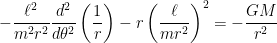
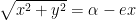
  , with the Sun at the origin, then under Newtonian mechanics (i.e., without general relativity) the motion of the planet follows the differential equation
 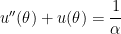 ,
, and
and  ,
, and the acceleration
  are vectors. When written in polar coordinates, this becomes
![{\bf F} = m \displaystyle \left[ \frac{d^2r}{dt^2} - r \left( \frac{d\theta}{dt} \right)^2 \right] {\bf u}_r + m \left(r \frac{d^2 \theta}{d t^2} + 2 \frac{dr}{dt} \frac{d\theta}{dt} \right) {\bf u}_\theta](https://s0.wp.com/latex.php?latex=%7B%5Cbf+F%7D+%3D+m+%5Cdisplaystyle+%5Cleft%5B+%5Cfrac%7Bd%5E2r%7D%7Bdt%5E2%7D+-+r+%5Cleft%28+%5Cfrac%7Bd%5Ctheta%7D%7Bdt%7D+%5Cright%29%5E2+%5Cright%5D+%7B%5Cbf+u%7D_r+%2B+m+%5Cleft%28r+%5Cfrac%7Bd%5E2+%5Ctheta%7D%7Bd+t%5E2%7D+%2B+2+%5Cfrac%7Bdr%7D%7Bdt%7D+%5Cfrac%7Bd%5Ctheta%7D%7Bdt%7D+%5Cright%29+%7B%5Cbf+u%7D_%5Ctheta&bg=ffffff&fg=000000&s=0&c=20201002) ,
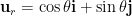
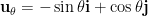
, is a unit vector pointing away from the origin and
  is a unit vector perpendicular to
  .
. ,
,![m \displaystyle \left[ \frac{d^2r}{dt^2} - r \left( \frac{d\theta}{dt} \right)^2 \right] = \displaystyle -\frac{GMm}{r^2}](https://s0.wp.com/latex.php?latex=m+%5Cdisplaystyle+%5Cleft%5B+%5Cfrac%7Bd%5E2r%7D%7Bdt%5E2%7D+-+r+%5Cleft%28+%5Cfrac%7Bd%5Ctheta%7D%7Bdt%7D+%5Cright%29%5E2+%5Cright%5D+%3D+%5Cdisplaystyle+-%5Cfrac%7BGMm%7D%7Br%5E2%7D&bg=ffffff&fg=000000&s=0&c=20201002) ,
, .
. ,
, .
.


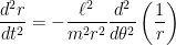
![\displaystyle \frac{\ell^2}{m^2 r^2} \left[ \frac{d^2}{d\theta^2} \left( \frac{1}{r} \right) + \frac{1}{r} \right] = \displaystyle \frac{GM}{r^2}](https://s0.wp.com/latex.php?latex=%5Cdisplaystyle++%5Cfrac%7B%5Cell%5E2%7D%7Bm%5E2+r%5E2%7D+%5Cleft%5B+%5Cfrac%7Bd%5E2%7D%7Bd%5Ctheta%5E2%7D+%5Cleft%28+%5Cfrac%7B1%7D%7Br%7D+%5Cright%29+%2B+%5Cfrac%7B1%7D%7Br%7D+%5Cright%5D++%3D+%5Cdisplaystyle+%5Cfrac%7BGM%7D%7Br%5E2%7D&bg=ffffff&fg=000000&s=0&c=20201002)
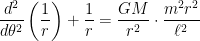
 .
. .
. as the constant on the right-hand side instead of just
  ,
, ,
, directors are
  and
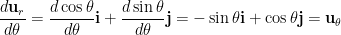
and  , and the unit vectors
  and
and  are perpendicular, pointing in the positive
  and positive
  directions.
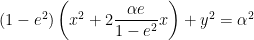
 . This may be rewritten as
 ,
,
 .
.
 .
. .
. .
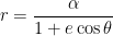
. , or a distance
  from the origin in the direction of
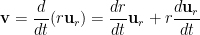

 .
.

![= \displaystyle \left[ \frac{d^2r}{dt^2} - r \left(\frac{d\theta}{dt} \right)^2 \right] {\bf u}_r + \left[ 2\frac{dr}{dt} \frac{d\theta}{dt} + r \frac{d^2\theta}{dt^2} \right] {\bf u}_\theta](https://s0.wp.com/latex.php?latex=%3D+%5Cdisplaystyle+%5Cleft%5B+%5Cfrac%7Bd%5E2r%7D%7Bdt%5E2%7D+-++r+%5Cleft%28%5Cfrac%7Bd%5Ctheta%7D%7Bdt%7D+%5Cright%29%5E2+%5Cright%5D+%7B%5Cbf+u%7D_r+%2B+%5Cleft%5B+2%5Cfrac%7Bdr%7D%7Bdt%7D+%5Cfrac%7Bd%5Ctheta%7D%7Bdt%7D+%2B+r+%5Cfrac%7Bd%5E2%5Ctheta%7D%7Bdt%5E2%7D+%5Cright%5D+%7B%5Cbf+u%7D_%5Ctheta&bg=ffffff&fg=000000&s=0&c=20201002) .
. ,
, ;
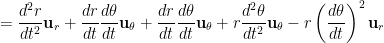
; in a form that depends only on


 .
. .
.


![= \displaystyle \frac{\ell}{mr^2} \frac{d}{d\theta} \left[ \frac{dr}{dt} \right]](https://s0.wp.com/latex.php?latex=%3D+%5Cdisplaystyle+%5Cfrac%7B%5Cell%7D%7Bmr%5E2%7D+%5Cfrac%7Bd%7D%7Bd%5Ctheta%7D+%5Cleft%5B+%5Cfrac%7Bdr%7D%7Bdt%7D+%5Cright%5D&bg=ffffff&fg=000000&s=0&c=20201002)
![= \displaystyle \frac{\ell}{mr^2} \frac{d}{d\theta} \left[ - \frac{\ell}{m} \frac{d}{d\theta} \left( \frac{1}{r} \right) \right]](https://s0.wp.com/latex.php?latex=%3D+%5Cdisplaystyle+%5Cfrac%7B%5Cell%7D%7Bmr%5E2%7D+%5Cfrac%7Bd%7D%7Bd%5Ctheta%7D+%5Cleft%5B+-+%5Cfrac%7B%5Cell%7D%7Bm%7D+%5Cfrac%7Bd%7D%7Bd%5Ctheta%7D+%5Cleft%28+%5Cfrac%7B1%7D%7Br%7D+%5Cright%29+%5Cright%5D&bg=ffffff&fg=000000&s=0&c=20201002)
![= \displaystyle - \frac{\ell^2}{m^2r^2} \frac{d}{d\theta} \left[ \frac{d}{d\theta} \left( \frac{1}{r} \right) \right]](https://s0.wp.com/latex.php?latex=%3D+%5Cdisplaystyle+-+%5Cfrac%7B%5Cell%5E2%7D%7Bm%5E2r%5E2%7D+%5Cfrac%7Bd%7D%7Bd%5Ctheta%7D+%5Cleft%5B+%5Cfrac%7Bd%7D%7Bd%5Ctheta%7D+%5Cleft%28+%5Cfrac%7B1%7D%7Br%7D+%5Cright%29+%5Cright%5D&bg=ffffff&fg=000000&s=0&c=20201002)
 .
.
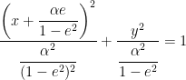
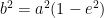
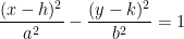
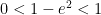
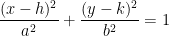
 . Furthermore, if
  , then this represents an ellipse with eccentricity
  whose major axis lies on the
  . Under this assumption,
  and
and  , so let me rewrite the previous equation in terms of
  :
:
 ,
,
 ,
,


 , this means that the origin is, once again, one of the foci of the hyperbola.
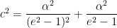
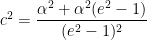
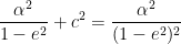
 of the hyperbola is easily computed as
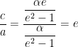 ,
,

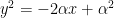
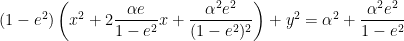
 . With this substitution, the equation in rectangular coordinates simplifies to
 .
. , so that
  . Then the equation in rectangular coordinates simplifies to
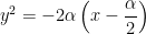

 .
. ,
, to the left of the vertex. In other words, the origin is the focus of the parabola. (For what it’s worth, the directrix of the parabola would be the vertical line
  , located
  to the right of the vertex.)
 .
.


 so that
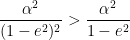 .
. ,
, ,
, ,
, .
. ,
,


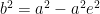
 . Therefore, since the foci of the ellipse are distance
  , or
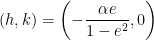
, or  . That is, the origin is one focus of the ellipse. (For the little it’s worth, the other focus is located at
  .
. .
. . For this ellipse, the planet’s closest approach to the Sun occurs at
 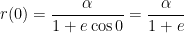 ,
, .
.

 .
. , we can also compute