In this series, I’m discussing how ideas from calculus and precalculus (with a touch of differential equations) can predict the precession in Mercury’s orbit and thus confirm Einstein’s theory of general relativity. The origins of this series came from a class project that I assigned to my Differential Equations students maybe 20 years ago.
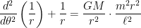
In this part of the series, we will show that if the motion of a planet around the Sun is expressed in polar coordinates  , with the Sun at the origin, then under Newtonian mechanics (i.e., without general relativity) the motion of the planet follows the differential equation
 ,
,
where  and
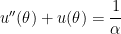
and  is a certain constant. Deriving this governing differential equation will require some principles from physics. If you’d rather skip the physics and get to the mathematics, we’ll get to solving this differential equations in the next post.
Part of the derivation of this governing differential equation will involve Newton’s Second Law
 ,
,
where  is the mass of the planet and the force
  and the acceleration
  are vectors. In usual rectangular coordinates, the acceleration vector would be expressed as
 ,
,
where the components of the acceleration in the  and
and  directors are
  and
and  , and the unit vectors
  and
and  are perpendicular, pointing in the positive
  and positive
  directions.
Unfortunately, our problem involves polar coordinates, and rewriting the acceleration vector in polar coordinates, instead of rectangular coordinates, is going to take some work.
Suppose that the position of the planet is in polar coordinates, so that the position in rectangular coordinates is  . This may be rewritten as
 ,
,
where
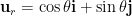
is a unit vector that points away from the origin. We see that this is a unit vector since
 .
.
We also define
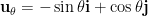
to be a unit vector that is perpendicular to  ; it turns out that
  points in the direction of increasing
  . To see that and are perpendicular, we observe
 .
.
Computing the velocity and acceleration vectors in polar coordinates will have a twist that’s not experienced with rectangular coordinates since both and are functions of . Indeed, we have
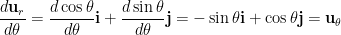 .
.
Furthermore,
 .
.
These two equations will be needed in the derivation below.
We are now in position to express the velocity and acceleration of the orbiting planet in polar coordinates. Clearly, the position of the planet is  , or a distance
  from the origin in the direction of . Therefore, by the Product Rule, the velocity of the planet is
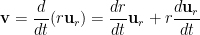
We now apply the Chain Rule to the second term:

 .
.
Differentiating a second time with respect to time, and again using the Chain Rule, we find


![= \displaystyle \left[ \frac{d^2r}{dt^2} - r \left(\frac{d\theta}{dt} \right)^2 \right] {\bf u}_r + \left[ 2\frac{dr}{dt} \frac{d\theta}{dt} + r \frac{d^2\theta}{dt^2} \right] {\bf u}_\theta](https://s0.wp.com/latex.php?latex=%3D+%5Cdisplaystyle+%5Cleft%5B+%5Cfrac%7Bd%5E2r%7D%7Bdt%5E2%7D+-++r+%5Cleft%28%5Cfrac%7Bd%5Ctheta%7D%7Bdt%7D+%5Cright%29%5E2+%5Cright%5D+%7B%5Cbf+u%7D_r+%2B+%5Cleft%5B+2%5Cfrac%7Bdr%7D%7Bdt%7D+%5Cfrac%7Bd%5Ctheta%7D%7Bdt%7D+%2B+r+%5Cfrac%7Bd%5E2%5Ctheta%7D%7Bdt%5E2%7D+%5Cright%5D+%7B%5Cbf+u%7D_%5Ctheta&bg=ffffff&fg=000000&s=0&c=20201002) .
.
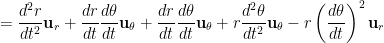
This will be needed in the next post, when we use both Newton’s Second Law and Newton’s Law of Gravitation, expressed in polar coordinates.


![{\bf F} = m \displaystyle \left[ \frac{d^2r}{dt^2} - r \left( \frac{d\theta}{dt} \right)^2 \right] {\bf u}_r + m \left(r \frac{d^2 \theta}{d t^2} + 2 \frac{dr}{dt} \frac{d\theta}{dt} \right) {\bf u}_\theta](https://s0.wp.com/latex.php?latex=%7B%5Cbf+F%7D+%3D+m+%5Cdisplaystyle+%5Cleft%5B+%5Cfrac%7Bd%5E2r%7D%7Bdt%5E2%7D+-+r+%5Cleft%28+%5Cfrac%7Bd%5Ctheta%7D%7Bdt%7D+%5Cright%29%5E2+%5Cright%5D+%7B%5Cbf+u%7D_r+%2B+m+%5Cleft%28r+%5Cfrac%7Bd%5E2+%5Ctheta%7D%7Bd+t%5E2%7D+%2B+2+%5Cfrac%7Bdr%7D%7Bdt%7D+%5Cfrac%7Bd%5Ctheta%7D%7Bdt%7D+%5Cright%29+%7B%5Cbf+u%7D_%5Ctheta&bg=ffffff&fg=000000&s=0&c=20201002)


![m \displaystyle \left[ \frac{d^2r}{dt^2} - r \left( \frac{d\theta}{dt} \right)^2 \right] = \displaystyle -\frac{GMm}{r^2}](https://s0.wp.com/latex.php?latex=m+%5Cdisplaystyle+%5Cleft%5B+%5Cfrac%7Bd%5E2r%7D%7Bdt%5E2%7D+-+r+%5Cleft%28+%5Cfrac%7Bd%5Ctheta%7D%7Bdt%7D+%5Cright%29%5E2+%5Cright%5D+%3D+%5Cdisplaystyle+-%5Cfrac%7BGMm%7D%7Br%5E2%7D&bg=ffffff&fg=000000&s=0&c=20201002)


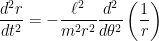
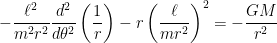


![\displaystyle \frac{\ell^2}{m^2 r^2} \left[ \frac{d^2}{d\theta^2} \left( \frac{1}{r} \right) + \frac{1}{r} \right] = \displaystyle \frac{GM}{r^2}](https://s0.wp.com/latex.php?latex=%5Cdisplaystyle++%5Cfrac%7B%5Cell%5E2%7D%7Bm%5E2+r%5E2%7D+%5Cleft%5B+%5Cfrac%7Bd%5E2%7D%7Bd%5Ctheta%5E2%7D+%5Cleft%28+%5Cfrac%7B1%7D%7Br%7D+%5Cright%29+%2B+%5Cfrac%7B1%7D%7Br%7D+%5Cright%5D++%3D+%5Cdisplaystyle+%5Cfrac%7BGM%7D%7Br%5E2%7D&bg=ffffff&fg=000000&s=0&c=20201002)


 Earth gravity. Hence, Earth’s well is 6,000 km deep.
 ,
,
 ,
, is the acceleration due to gravity near Earth’s surface. Also, work equals force times distance. Therefore, if the rocket travels a distance
  against this (hypothetically) constant gravity, then
 .
. .
. over 3 days (accounting for roundoff error in the last decimal place), and so the average rate of change is
 .
. ,
, is the
  is the mass of the beer keg,
  is the distance of a particle from the center of the beer keg,
  .
. .
. .
.