From Wikipedia, Lagrange points are points of equilibrium for small-mass objects under the gravitational influence of two massive orbiting bodies. There are five such points in the Sun-Earth system, called , , , , and .
The stable equilibrium points and are easiest to explain: they are the corners of equilateral triangles in the plane of Earth’s orbit. The points and are also equilibrium points, but they are unstable. Nevertheless, they have practical applications for spaceflight.
As we’ve seen, the positions of and can be found by numerically solving the fifth-order polynomial equations
and
,
respectively. In these equations, where is the mass of the Sun and is the mass of Earth. Also, is the distance from the Earth to or measured as a proportion of the distance from the Sun to Earth.
We’ve also seen that, for the Sun and Earth, , and numerically solving the above quintics yields for and for . In other words, and are approximately the same distance from Earth but in opposite directions.
There’s a good reason why the positive real roots of these two similar quintics are almost equal. We know that will be a lot closer to 0 than 1 because, for gravity to balance, the Lagrange points have to be a lot closer to Earth than the Sun. For this reason, the terms and will be a lot smaller than , and so those two terms can be safely ignored in a first-order approximation. Also, the terms and will be a lot smaller than , and so those two terms can also be safely ignored in a first-order approximation. Furthermore, since is also close to 0, the coefficient can be safely replaced by just .
Consequently, the solution of both quintic equations should be close to the solution of the cubic equation
,
which is straightforward to solve:
.
If , we obtain , which is indeed reasonably close to the actual solutions for and . Indeed, this may be used as the first approximation in Newton’s method to quickly numerically evaluate the actual solutions of the two quintic polynomials.
In this series, I’m discussing how ideas from calculus and precalculus (with a touch of differential equations) can predict the precession in Mercury’s orbit and thus confirm Einstein’s theory of general relativity. The origins of this series came from a class project that I assigned to my Differential Equations students maybe 20 years ago.
One technique that will be necessary for this confirmation is the method of successive approximations. This will be needed in the context of a differential equation; however, we can illustrate the concept by finding the roots of a polynomial. Consider the quadratic equation
.
(Naturally, we can solve for using the quadratic formula; more on that later.) To apply the method of successive approximation, we will rewrite this so that appears on the left side and some function of appears on the right side. I will choose
, or
.
Here’s the idea of the method of successive approximations to obtain a recursively defined sequence that (hopefully) convergence to a solution of this equation:
Start with an initial guess .
Plug into the right-hand side to get a new guess, .
Plug into the right-hand side to get a new guess, .
And repeat.
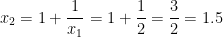
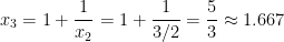
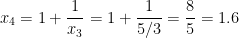
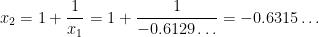
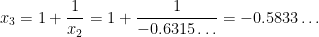
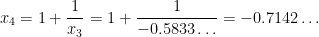
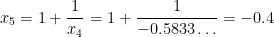
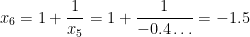
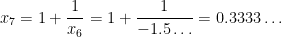
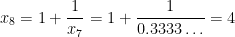
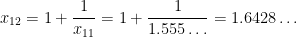
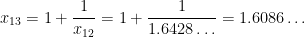
For example, suppose that we choose . Then
This sequence can be computed by entering into a calculator, then entering , and then repeatedly hitting the button.
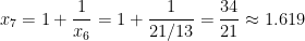
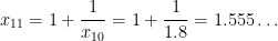
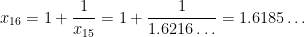
We see that the sequence appears to be converging to something, and that something is a root of the equation , which we now find via the quadratic formula:
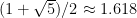
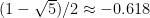
.
So it looks like the above sequence is converging to the positive root .
(Parenthetically, you might notice that the Fibonacci sequence appears in the numerators and denominators of this sequence. As you might guess, that’s not a coincidence.)
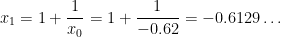
Like most numerical techniques, this method doesn’t always work like we think it would. Another solution is the negative root . Unfortunately, if we start with a guess near this root, like , the sequence unexpectedly diverges from but eventually converges to the positive root :
I should note that the method of successive approximations generally converges at a slower pace than Newton’s method. However, this method will be good enough when we use it to predict the precession in Mercury’s orbit.
This is the last in a series of posts about square roots and other roots, hopefully providing a deeper look at an apparently simple concept. However, in this post, we discuss how calculators are programmed to compute square roots quickly.
Today’s movie clip, therefore, is set in modern times:
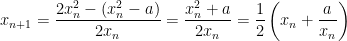
So how do calculators find square roots anyway? First, we recognize that is a root of the polynomial . Therefore, Newton’s method (or the Newton-Raphson method) can be used to find the root of this function. Newton’s method dictates that we begin with an initial guess and then iteratively find the next guesses using the recursively defined sequence
For the case at hand, since , we may write
,
which reduces to
This algorithm can be programmed using C++, Python, etc.. For pedagogical purposes, however, I’ve found that a spreadsheet like Microsoft Excel is a good way to sell this to students. In the spreadsheet below, I use Excel to find . In cell A1, I entered as a first guess for . Notice that this is a really lousy first guess! Then, in cell A2, I typed the formula
=1/2*(A1+2000/A1)
So Excel computes
.
Then I filled down that formula into cells A3 through A16.
Notice that this algorithm quickly converges to , even though the initial guess was terrible. After 7 steps, the answer is only correct to 2 significant digits (). After 8 steps, the answer is correct to 4 significant digits (). On the 9th step, the answer is correct to 9 significant digits ().
Indeed, there’s a theorem that essentially states that, when this algorithm converges, the number of correct digits basically doubles with each successive step. That’s a lot better than the methods shown at the start of this series of posts which only produced one extra digit with each step.
This algorithm works for finding th roots as well as square roots. Since is a root of , Newton’s method reduces to
,
which reduces to the above sequence if .
See also this Wikipedia page for further historical information as well as discussion about how the above recursive sequence can be obtained without calculus.


![t = \displaystyle \sqrt[3]{ \frac{\mu}{3} }](https://s0.wp.com/latex.php?latex=t+%3D+%5Cdisplaystyle+%5Csqrt%5B3%5D%7B+%5Cfrac%7B%5Cmu%7D%7B3%7D+%7D&bg=ffffff&fg=000000&s=0&c=20201002)


 .
. using the quadratic formula; more on that later.) To apply the method of successive approximation, we will rewrite this so that
  , or
, or .
. .
. .
. .
. . Then


 into a calculator, then entering
  , and then repeatedly hitting the
  button.
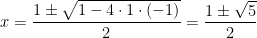 .
. .
.
 . Unfortunately, if we start with a guess near this root, like
  , the sequence unexpectedly diverges from
  but eventually converges to the positive root
  :
:


 is a root of the polynomial
  . Therefore,
 , we may write
 ,
,
 . In cell A1, I entered
  as a first guess for
 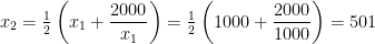 .
.
 ). After 8 steps, the answer is correct to 4 significant digits (
 ). On the 9th step, the answer is correct to 9 significant digits (
 ).
). th roots as well as square roots. Since
 ![\sqrt[k]{a}](https://s0.wp.com/latex.php?latex=%5Csqrt%5Bk%5D%7Ba%7D&bg=ffffff&fg=000000&s=0&c=20201002) is a root of
is a root of  , Newton’s method reduces to
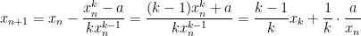 ,
, .
.