Engaging students: Powers and exponents

In my capstone class for future secondary math teachers, I ask my students to come up with ideas for engaging their students with different topics in the secondary mathematics curriculum. In other words, the point of the assignment was not to devise a full-blown lesson plan on this topic. Instead, I asked my students to think about three different ways of getting their students interested in the topic in the first place.

I plan to share some of the best of these ideas on this blog (after asking my students’ permission, of course).

This student submission comes from my former student Kayla (Koenig) Lambert. Her topic, from Pre-Algebra: powers and exponents.

A) Applications: What interesting word problems using this topic can your students do now?

I chose the problem below from http://www.purplemath.com because I think that solving a problem that deals with disease would be interesting to my students. People have to deal with sickness and disease everyday and I think that solving a real world problem would entice the students into wanting to learn more.

A biologist is researching a newly-discovered species of bacteria. At time t = 0 hours, he puts one hundred bacteria into what he has determined to be a favorable growth medium. Six hours later, he measures 450 bacteria. Assuming exponential growth, what is the growth constant “k” for the bacteria? (Round k to two decimal places.)

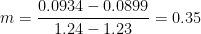
For this exercise, the units on time t will be hours, because the growth is being measured in terms of hours. The beginning amount P is the amount at time t = 0, so, for this problem, P = 100. The ending amount is A = 450 at t = 6. The only variable I don’t have a value for is the growth constant k, which also happens to be what I’m looking for. So I’ll plug in all the known values, and then solve for the growth constant:

$A = Pe^{kt}$

$450 = 100 e^{6k}$

$4.5 = e^{6k}$

$\ln(4.5) = 6k$

$k = \displaystyle \frac{\ln(4.5)}{6} = 0.250679566129\dots$

The growth constant is 0.25/hour.

I think this kind of problem would be beneficial to students because it would help them understand how bacteria grows and how easily they can get catch something and get sick.

C) Culture: How has this topic appeared in pop culture?

Exponents and powers are everywhere around us without the students knowledge. Many movies and video games have ideas related to powers and exponents. Take, for example, the movie Contagion that was released in September 2011. This movie is about “the threat posed by a deadly disease and an international team of doctors contracted by the CDC to deal with the outbreak” (http://www.imdb.com/title/tt1598778). In this movie, there is a scene where the doctors are using mathematical equations with exponents to find out how fast the disease spreads and how much time they have left to save the majority of the population. There are many movies like this that involve powers and exponents, Contagion is just one example. There are also popular video games that deal with the spread of disease. For example, in the video game Call Of Duty: World At War the player is a soldier in WWII and his mission is to kill zombies, and zombie populations grow exponentially. Now, my brother plays this game and I know for a fact that he doesn’t think about the mathematics behind it, but I think talking about pop culture while teaching would really bring some excitement to the classroom and get the students thinking.

D) History: Who were some of the people who contributed to the discovery of this topic?

Exponents and powers have been among humans since the time of the Babylonians in Egypt. “Babylonians already knew the solution to quadratic equations and equations of the second degree with two unknowns and could also handle equations to the third and fourth degree” (Mathematics History). The Egyptians also had a good idea about powers and exponents around 3400 BC. They used their “hieroglyphic numeral system” which was based on the scale of 10. When using their system, the Egyptians expressed any number using their symbols, with each symbol being “repeated the required number of times” (Mathematics History). However, the first actual recorded use of powers and exponents was in a book called “Artihmetica Integra” written by English author and Mathematician Michael Stifel in 1544 (History of Exponents). In the 14^th century Nicole Oresme used “numbers to indicate powering”(Jeff Miller Pages). Also, James Hume used Roman Numerals as exponents in the book L’Algebre de Viete d’vne Methode Novelle in 1636. Exponents were used in modern notation be Rene Descartes in 1637. Also, negative integers as exponents were “first used in modern notation” by Issac Newton in 1676 (Jeff Miller Pages).

Works Cited

Ayers, Chuck. “The History of Exponents | eHow.com.” eHow | How to Videos, Articles & More – Discover the expert in you. | eHow.com. N.p., n.d. Web. 25 Jan. 2012. http://www.ehow.com/about_5134780_history-exponents.html.

“Contagion (2011) – IMDb.” The Internet Movie Database (IMDb). N.p., n.d. Web. 25 Jan. 2012. http://www.imdb.com/title/tt1598778/.

“Exponential Word Problems.” Purplemath. N.p., n.d. Web. 25 Jan. 2012. http://www.purplemath.com/modules/expoprob2.htm.

“Mathematics History.” ThinkQuest : Library. N.p., n.d. Web. 25 Jan. 2012. http://library.thinkquest.org/22584/.

juxtaposition.. “Earliest Uses of Symbols of Operation.” Jeff Miller Pages. N.p., n.d. Web. 25 Jan. 2012. http://jeff560.tripod.com/operation.html.

Square roots and logarithms without a calculator (Part 9)

This post is not really about finding square roots but continues Part 8 of this series. Continuing the theme of this series, let’s go back in time to when scientific calculators were not invented… say, 1850.

This is a favorite activity that I use when teaching logarithms to precalculus students. I begin by writing the following on the board, in three or four columns:

$\log_{10} 1$

$\log_{10} 2 \approx 0.301$

$\log_{10} 3 \approx 0.477$

$\log_{10} 4$

$\log_{10} 5$

$\log_{10} 6$

$\log_{10} 7$

$\log_{10} 8$

$\log_{10} 9$

$\log_{10} 10$

$\log_{10} 11$

$\log_{10} 12$

$\log_{10} 13$

$\log_{10} 14$

$\log_{10} 15$

$\log_{10} 16$

$\log_{10} 17$

$\log_{10} 18$

$\log_{10} 19$

$\log_{10} 20$

$\log_{10} 30$

$\log_{10} 40$

$\log_{10} 50$

$\log_{10} 60$

$\log_{10} 70$

$\log_{10} 80$

$\log_{10} 90$

$\log_{10} 100$

In other words, I tell the answer to only $\log_{10} 2$ and $\log_{10} 3$ . The challenge: fill in the rest without a calculator.

In my classes, we found these logarithms by large-group discussion. However, there’s no reason why this couldn’t be done by dividing a class into small groups and letting the groups collaborate. Indeed, I suggested this idea to a former student who was struggling to come up with an engaging activity involving logarithms for an Algebra II class that she was about to teach. She took this idea and ran with it, and she told me it was a big hit with her students.

I provide a thought bubble if you’d like to think about it before I give the answers.

Step 1. Three of these values — $1$ , $10$ , and $100$ — can be found exactly since they’re powers of $10$ .

Step 2. Most of the others can be found by using the laws of logarithms for products, quotients, and powers involving $2$ , $3$ , and $10$ . For example,

$\log_{10} 9 = \log_{10} 3^2 = 2 \log_{10} 3 \approx 2 \times 0.477 = 0.954$

$\log_{10} 20 = \log_{10} 2 + \log_{10} 10 = 1.301$

$\log_{10} 5 = \log_{10} 10 - \log_{10} 2 = 0.699$ .

Of this group, usually $\log_{10} 5$ is the hardest for students to recognize.

Step 3 (optional). A few of the logarithms, like $\log_{10} 7$ , cannot be determined in terms of $\log_{10} 2$ and $\log_{10} 3$ . But they can be approximated to reasonable accuracy with a little creativity. For example,

$\log_{10} 7 = \log_{10} \sqrt{49} = \frac{1}{2} \log_{10} 49 \approx \frac{1}{2} \log_{10} 50 = \frac{1}{2} (1.699) = 0.850$ .

For a really good approximation, we use the fact that $7^4 = 2401 \approx 2400$ .

$\log_{10} 7 = \frac{1}{4} \log_{10} 2401 \approx \frac{1}{4} \log_{10} 2400 = \frac{1}{4} (3 \log_{10} 2 + \log_{10} 3 + \log_{10} 100) = 0.845$ .

To approximate $\log_{10} 17$ , we could use the fact that $(16-1) \times (16 + 1) = 16^2-1$ , or $15 \times 17 = 255 \approx 2^8$ . So

$\log_{10} 17 \approx 8 \log_{10} 2 - \log_{10} 15 = 8 \log_{10} 2 - \log_{10} 3 - \log_{10} 5 = 1.232$

Naturally, any and all of the above results can be confirmed with a scientific calculator.

In my opinion, here are some of the pedagogical benefits of the above activity.

1. This activity solidifies students’ knowledge about the laws of logarithms. The laws of logarithms become less abstract, changing from $\log_{10} xy = \log_{10} x + \log_{10} y$ into something more tangible and comfortable, like positive integers.

2. Hopefully the activity will demystify for students the curious decimal expansions when a calculator returns logarithms. In other words, hopefully the above activity will help

3. The activity should promote some understanding of the values of base-10 logarithms. For example, $0 \le \log_{10} x < 1$ for $1 \le x < 10$ and $1 \le \log_{10} x < 2$ for $10 \le x < 100$ .

4. Students should see that, for large $x$ , $\log_{10}(x+1)$ is not much larger than $\log_{10} x$ . This is another way of saying that the graph of $y = \log_{10} x$ increases very slowly as $x$ increases. So this should provide some future intuition for the graphs of logarithmic functions.

5. The values of $\log_{10} 2, \log_{10} 3, \dots, \log_{10} 9$ are used to construct the unevenly-spaced lines and/or tick marks in log-log graphs and log-linear graphs (which are standard plotting options on many scientific calculators).

Square roots and logarithms without a calculator (Part 8)

I’m in the middle of a series of posts concerning the elementary operation of computing a root. This is such an elementary operation because nearly every calculator has a $\sqrt{~~}$ button, and so students today are accustomed to quickly getting an answer without giving much thought to (1) what the answer means or (2) what magic the calculator uses to find roots. I like to show my future secondary teachers a brief history on this topic… partially to deepen their knowledge about what they likely think is a simple concept, but also to give them a little appreciation for their elders.

To begin, let’s again go back to a time before the advent of pocket calculators… say, 1952.

This story doesn’t go back to 1952 but to Boxing Day 2012 (the day after Christmas). For some reason, my daughter — out of the blue — asked me to compute $\sqrt[19]{25727}$ without a calculator. As my daughter adores the ground I walk on — and I want to maintain this state of mind for as long as humanly possible — I had no choice but to comply. So I might as well have been back in 1952.

In the past few posts, I discussed how log tables and slide rules were used by previous generations to perform this calculation. The problem was that all of these tools were in my office and not at home, and hence were not of immediate use.

The good news is that I had a few logarithms memorized:

$\log_{10} 2 \approx 0.301$ , $\log_{10} 3 \approx 0.477$ , $\log_{10} 7 = 0.845$ ,

and $\ln 10 = 2.3$ .

I had the first two logs memorized when I was a child; the third I memorized later. As I’ll describe, the first three logarithms can be used with the laws of logarithms to closely approximate the base-10 logarithm of nearly any number. The last logarithm was important in previous generations for using the change-of-base formula from $\log_{10}$ to $\ln$ . It was also prominently mentioned in the chapter “Lucky Numbers” from a favorite book of my childhood, Surely You’re Joking Mr. Feynman, so I had that memorized as well.

I also knew that $\ln(1+x) \approx x$ for $x = 0$ from the Taylor expansion of $\ln(1+x)$ .

To begin, I first noticed that $25727 \approx 25600$ , and I knew I could get $\log_{10} 25600$ since $25600 = 2^8 \times 100$ . So I started with

$\log_{10} 25727 = \log_{10} \left(100 \times 256 \times \displaystyle \frac{257.27}{256} \right)$

$\log_{10} 25727 \approx \log_{10} 100 + 8 \log_{10} 2 + \log_{10} 1.005$

$\log_{10} 25727 \approx 2 + 8(0.301) + \displaystyle \frac{\ln 1.005}{\ln 10}$

$\log_{10} 25727 \approx 4.408 + \displaystyle \frac{0.005}{2.3}$

$\log_{10} 25727 \approx 4.408 + 0.002$

$\log_{10} 25727 \approx 4.410$

I did all of the above calculations by hand, cutting off after three decimal places (since I had those base-10 logarithms memorized to only three decimal places). Therefore,

$\log_{10} 25727^(1/19) = \displaystyle \frac{1}{19} \log_{10} 25727 \approx \displaystyle \frac{4.410}{19} \approx 0.232$

So, to complete the calculation, I had to find the value of $x$ so that $\log_{10} x = 0.232$ . This was by far the hardest step, since it could only be done by trial and error. I forget exactly what steps I tried, but here’s a sample:

$\log_{10} 2 \approx 0.301$ . Too big.

$\log_{10} 1.5 = \log_{10} \displaystyle \frac{3}{2} = \log_{10} 3 - \log_{10} 2 \approx 0.477 - 0.301 = 0.176$ . Too small.

$\log_{10} 1.6 = \log_{10} \displaystyle \frac{2^4}{10} = 4\log_{10} 2 - \log_{10} 10 \approx 4(0.301) - 1 = 0.203$ . Too small.

$\log_{10} 1.8 = \log_{10} \displaystyle \frac{2 \cdot 3^2}{10} \approx 0.301 + 2(0.477) - 1 = 0.255$ . Too big.

Eventually, I got to

$\log_{10} 1.71 = \log_{10} \displaystyle \frac{3^2 \cdot 19}{100}$

$\log_{10} 1.71 = 2\log_{10} 3 + \log_{10} 19 - \log_{10} 100$

$\log_{10} 1.71 \approx 2(0.477) + \displaystyle \frac{\log_{10} 18 + \log_{10} 20}{2} - 2$

$\log_{10} 1.71 \approx -1.046 + \frac{1}{2} (\log_{10} 2 + 2 \log_{10} 3 + \log_{10} 2 + \log_{10} 10)$

$\log_{10} 1.71 \approx -1.046 + \frac{1}{2}(2.556)$

$\log_{10} 1.71 \approx 0.232$

So, after a hour or two of arithmetic, I told her my answer: $\sqrt[19]{25727} \approx 1.71$ . You can imagine my sheer delight when we checked my answer with a calculator:

In Part 9, I’ll discuss my opinion about whether or not these kinds of calculations have any pedagogical value for students learning logarithms.

Square roots and logarithms without a calculator (Part 7)

I’m in the middle of a series of posts concerning the elementary operation of computing a square root. This is such an elementary operation because nearly every calculator has a $\sqrt{~~}$ button, and so students today are accustomed to quickly getting an answer without giving much thought to (1) what the answer means or (2) what magic the calculator uses to find square roots. I like to show my future secondary teachers a brief history on this topic… partially to deepen their knowledge about what they likely think is a simple concept, but also to give them a little appreciation for their elders.

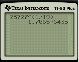
Today’s topic — slide rules — not only applies to square roots but also multiplication, division, and raising numbers to any exponent (not just to the $1/2$ power). To begin, let’s again go back to a time before the advent of pocket calculators… say, the 1950s.

Nearly all STEM professionals were once proficient in the use of slide rules. I never learned how to use one as a student. As a college professor, I bought a fairly inexpensive one from Slide Rule Universe. If you’ve never seen a slide rule, here’s a picture of a fairly advanced one. There are multiple rows of numbers and a sliding plastic piece that has a thin vertical line, allowing direct correspondence from one row of numbers to another. (The middle rows are on a piece that slides back and forth; this is necessary for doing multiplication and division with a slide rule.)

Let’s repeat the problem from Part 6 and try to find

$\log_{10} x = \log_{10} \sqrt{4213} = \log_{10} (4213)^{1/2} = \displaystyle \frac{1}{2} \log_{10} 4213$ .

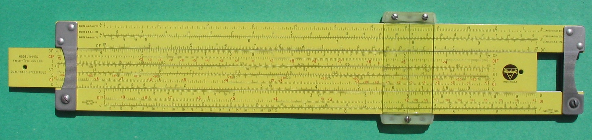
We recall that $\log_{10} 4213 = 3 + \log_{10} 4.213$ . The logarithm on the right-hand side can be estimated by looking at a slide rule. Here’s a picture from my slide rule:

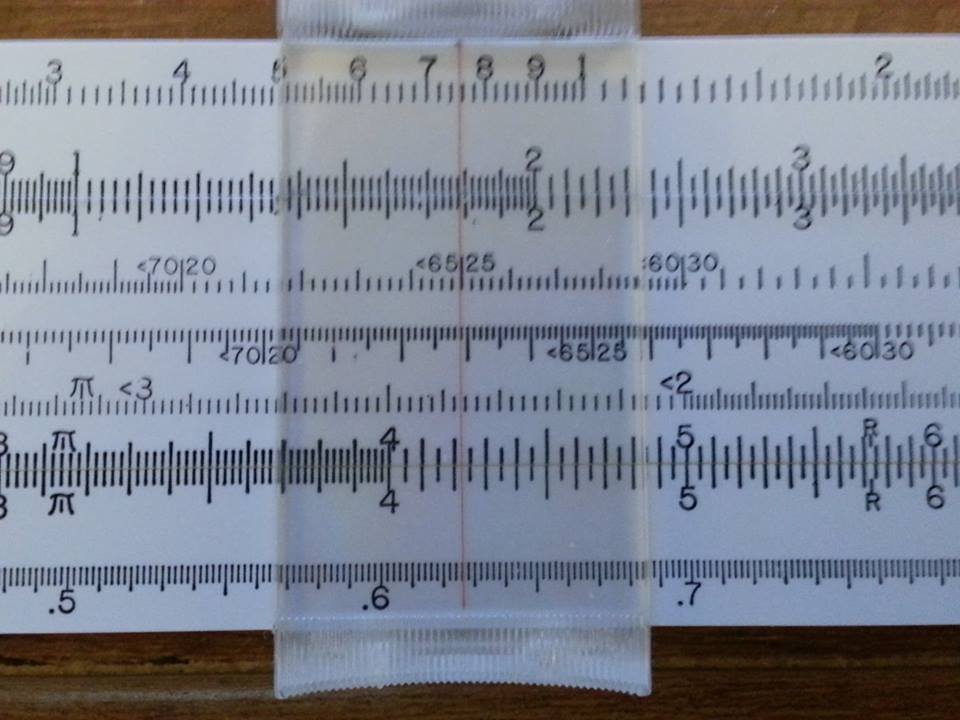
The important parts of this picture are the bottom two rows. Note that the thin red line is lined up between $4.2$ and $4.25$ ; indeed, the red line is about one-third of way from $4.2$ to $4.25$ . On the bottom row, the thin red line is lined up with $0.626$ . So we estimate that $\log_{10} 4213 \approx 3.626$ , so that $\log_{10} \sqrt{4213} \approx \frac{1}{2} (3.626) = 1.813$ .

Working the other direction, we must find $10^{1.813} = 10 \times 10^{0.813}$ . We move the thin red line to a different part of the slide rule:

This time, the thin red line is lined up with $0.813$ on the bottom row. On the row above, the red line is lined up almost exactly on $6.5$ , but perhaps a little to the left of $6.5$ . So we estimate that $10^{1.813} \approx 64.9$ or $64.95$ .

The correct answer is $64.907\dots$ .

Not bad for a piece of plastic.

Because taking square roots is so important, many slide rules have lines that simulate a square-root function… without the intermediate step of taking logarithms. Let’s consider again at the above picture, but this time let’s look at the second row from the top. Notice that the thin red line goes between $42$ and $42.5$ on the second line. (FYI, the line repeats itself to the left, so that the user can tell the difference between $42$ and $4.2$ .) Then looking down to the second line from the bottom, we see that the square root is a little less than $65$ , as before.

In addition to square roots, my personal slide rule has lines for cube roots, sines, cosines, and tangents. In the past, more expensive slide rules had additional lines for the values of other mathematical functions.

Square roots and logarithms without a calculator (Part 6)

In Parts 3-5 of this series, I discussed how log tables were used in previous generations to compute logarithms and antilogarithms.

Today’s topic — log tables — not only applies to square roots but also multiplication, division, and raising numbers to any exponent (not just to the $1/2$ power). After showing how log tables were used in the past, I’ll conclude with some thoughts about its effectiveness for teaching students logarithms for the first time.

To begin, let’s again go back to a time before the advent of pocket calculators… say, the 1880s.

Aside from a love of the movies of both Jimmy Stewart and John Wayne, I chose the 1880s on purpose. By the end of that decade, James Buchanan Eads had built a bridge over the Mississippi River and had designed a jetty system that allowed year-round navigation on the Mississippi River. Construction had begun on the Panama Canal. In New York, the Brooklyn Bridge (then the longest suspension bridge in the world) was open for business. And the newly dedicated Statue of Liberty was welcoming American immigrants to Ellis Island.

And these feats of engineering were accomplished without the use of pocket calculators.

Here’s a perfectly respectable way that someone in the 1880s could have computed $\sqrt{4213}$ to reasonably high precision. Let’s write

$x = \sqrt{4213}$ .

Take the base-10 logarithm of both sides.

$\log_{10} x = \log_{10} \sqrt{4213} = \log_{10} (4213)^{1/2} = \displaystyle \frac{1}{2} \log_{10} 4213$ .

Then log tables can be used to compute $\log_{10} 4213$ .

Step 1. In our case, we’re trying to find $\log_{10} 4213$ . We know that $\log_{10} 1000 = 3$ and $\log_{10} 10,000 = 4$ , so the answer must be between $3$ and $4$ . More precisely,

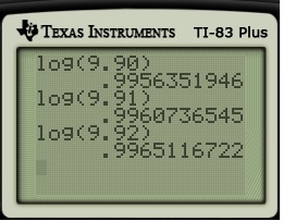
$\log_{10} 4213 = \log_{10} (1000 \times 4.213) = \log_{10} 1000 + \log_{10} 4.213 = 3 + \log_{10} 4.213$ .

To find $\log_{10} 4.213$ , we see from the table that

$\log_{10} 4.21 \approx 0.6243$ and $\log_{10} 4.22 = 0.6253$

So, to estimate $\log_{10} 4.213$ , we will employ linear interpolation. That’s a fancy way of saying “Find the line connecting $(4.21,0.6243)$ and $(4.22,0.6253)$ , and find the point on the line whose $x-$ coordinate is $4.213$ . Finding this line is a straightforward exercise in the point-slope form of a line:

$m = \displaystyle \frac{0.6253-0.6243}{4.22-4.21} = 0.1$

$y - 0.6243 = 0.1 (x - 4.21)$

$y = 0.6243 + 0.1 (4.213-4.21)$

$y = 0.6243 + 0.1(0.003) = 0.6246$

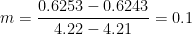
So we estimate $\log_{10} 4.213 \approx 0.6246$ . Thus, so far in the calculation, we have

$\log_{10} \sqrt{4213} \approx \displaystyle \frac{1}{2} (3 + 0.6246) = 1.8123$

Step 2. We then take the antilogarithm of both sides. The term antilogarithm isn’t used much anymore, but the principle is still taught in schools: take $10$ to the power of both the left- and right-hand sides. We obtain

$\sqrt{4213} \approx 10^{1.8123} = 10^{1 + 0.8123} = 10^1 \times 10^{0.8123}$

The first part of the right-hand side is easy: $10^1 = 10$ . For the second-part, we use the log table again, but in reverse. We try to find the numbers that are closest to $0.8123$ in the body of the table. In our case, we find that

$\log_{10} 6.49 = 0.8122$ and $\log_{10} 6.50 = 0.8129$ .

Once again, we use linear interpolation to find the line connecting $(6.49,0.8122)$ and $(6.50,0.8129)$ , except this time the $y-$ coordinate of $0.8123$ is known and the $x-$ coordinate is unknown.

$m = \displaystyle \frac{0.8129-0.8122}{6.50-6.49} = 0.07$

$y - 0.8122 = 0.07 (x - 6.49)$

$0.8123 - 0.8122 = 0.07 (x - 6.49)$

$x = 6.49 + \displaystyle \frac{0.0001}{0.07} = 6.4914\dots$

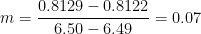
Since the table is only accurate to four significant digits, we estimate that $10^{0.8123} \approx 6.491$ . Therefore,

$\sqrt{4213} \approx 10^1 \times 10^{0.8123} = 10 \times 6.491 = 64.91$

By way of comparison, the answer is $\sqrt{4213} \approx 64.9076\dots \approx 64.91$ , rounding at the hundredths digit. Not bad, for a generation born before the advent of calculators.

With a little practice, one can do the above calculations with relative ease. Also, many log tables of the past had a column called “proportional parts” that essentially replaced the step of linear interpolation, thus speeding the use of the table considerably.

Log tables can be used for calculations more complex than finding a square root. For example, suppose I need to calculate

$x = \displaystyle \frac{(34.5)^3}{(912)^{2/5}}$

Using the log table, and without using a calculator, I find that

$\log_{10} x = 3 \log_{10} 34.5 - \displaystyle \frac{2}{5} \log_{10} 912$

$\log_{10} x = 3(1.5378) - \displaystyle \frac{2}{5} (2.9600)$

$\log_{10} x = 3.4294$

$x = 10^3 \cdot 10^{0.4294} = 1000 \cdot 2.688 = 2688$

That’s the correct answer to four significant digits. Using a calculator, we find the answer is $2688.186\dots$

Square roots and logarithms without a calculator (Part 5)

One way that square roots can be computed without a calculator is by using log tables. This was a common computational device before pocket scientific calculators were commonly affordable… say, the 1920s.

As many readers may be unfamiliar with this blast from the past, Parts 3 and 4 of this series discussed the mechanics of how to use a log table. In Part 6, I’ll discuss how square roots (and other operations) can be computed with using log tables.

In this post, I consider the modern pedagogical usefulness of log tables, even if logarithms can be computed more easily with scientific calculators.

A personal story: In either 1981 or 1982, my parents bought me my first scientific calculator. It was a thing of beauty… maybe about 25% larger than today’s TI-83s, with an LED screen that tilted upward. When it calculated something like $\log_{10} 4213$ , the screen would go blank for a couple of seconds as it struggled to calculate the answer. I’m surprised that smoke didn’t come out of both sides as it struggled. It must have cost my parents a small fortune, maybe over $1000 after adjusting for inflation. Naturally, being an irresponsible kid in the early 1980s, it didn’t last but a couple of years. (It’s a wonder that my parents didn’t kill me when I broke it.)

So I imagine that requiring all students to use log tables fell out of favor at some point during the 1980s, as technology improved and the prices of scientific calculators became more reasonable.

I regularly teach the use of log tables to senior math majors who aspire to become secondary math teachers. These students who have taken three semesters of calculus, linear algebra, and several courses emphasizing rigorous theorem proving. In other words, they’re no dummies. But when I show this blast from the past to them, they often find the use of a log table to be absolutely mystifying, even though it relies on principles — the laws of logarithms and the point-slope form of a line — that they think they’ve mastered.

So why do really smart students, who after all are math majors about to graduate from college, struggle with mastering log tables, a concept that was expected of 15- and 16-year-olds a generation ago? I personally think that a lot of their struggles come from the fact that they don’t really know logarithms in the way that students of previous generation had to know them in order to survive precalculus. For today’s students, a logarithm is computed so easily that, when my math majors were in high school, they were not expected to really think about its meaning.

For example, it’s no longer automatic for today’s math majors to realize that $\log_{10} 4213$ has to be between $3$ and $4$ someplace. They’ll just punch the numbers in the calculators to get an answer, and the process happens so quickly that the answer loses its meaning.

They know by heart that $\log_{b} xy = \log_{b} x + \log_{b} y$ and that $\log_b b^x = x$ . But it doesn’t reflexively occur to them that these laws can be used to rewrite $\log_{10} 4213$ as $3 + \log_{10} 4.213$ .

When encountering $10^{1.8123}$ , their first thought is to plug into a calculator to get the answer, not to reflect and realize that the answer, whatever it is, has to be between $10$ and $100$ someplace.

Today’s math majors can be taught these approximation principles, of course, but there’s unfortunately no reason to expect that they received the same training with logarithms that students received a generation ago. So none of this discussion should be considered as criticism of today’s math majors; it’s merely an observation about the training that they received as younger students versus the training that previous generations received.

So, do I think that all students today should exclusively learn how to use log tables? Absolutely not.If college students who have received excellent mathematical training can be daunted by log tables, you can imagine how the high school students of generations past must have felt — especially the high school students who were not particularly predisposed to math in the first place.

People like me that made it through the math education system of the 1980s (and before) received great insight into the meaning of logarithms. However, a lot of students back then found these tables as mystifying as today’s college students, and perhaps they did not survive the system because they found the use of the table to be exceedingly complex. In other words, while they were necessary for an era that pre-dated pocket calculators, log tables (and trig tables) were an unfortunate conceptual roadblock to a lot of students who might have had a chance at majoring in a STEM field. By contrast, logarithms are found easily today so that the steps above are not a hindrance to today’s students.

That said, I do argue that there is pedagogical value (as well as historical value) in showing students how to use log tables, even though calculators can accomplish this task much quicker. In other words, I wouldn’t expect students to master the art of performing the above steps to compute logarithms on the homework assignments and exams. But if they can’t perform the above steps, then there’s room for their knowledge of logarithms to grow.

And it will hopefully give today’s students a little more respect for their elders.

Square roots and logarithms without a calculator (Part 4)

I’m in the middle of a series of posts concerning the elementary operation of computing a square root. In Part 3 of this series, I discussed how previous generations computed logarithms without a calculator by using log tables. In this post, I’ll discuss how previous generations computed, using the language of the time, antilogarithms. In Part 5, I’ll discuss my opinions about the pedagogical usefulness of log tables, even if logarithms can be computed more easily with scientific calculators. And in Part 6, I’ll return to square roots — specifically, how log tables can be used to find square roots.

Let’s again go back to a time before the advent of pocket calculators… say, 1943.

The following log tables come from one of my prized possessions: College Mathematics, by Kaj L. Nielsen (Barnes & Noble, New York, 1958).

How to use the table, Part 5. The table can also be used to work backwards and find an antilogarithm. The term antilogarithm isn’t used much anymore, but the principle is still used in teaching students today. Suppose we wish to solve

$\log_{10} x = 0.9509$ , or $x = 10^{0.9509}$ .

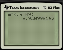
Looking through the body of the table, we see that $9509$ appears on the row marked $89$ and the column marked $3$ . Therefore, $10^{0.9509} \approx 8.93$. Again, this matches (to three and almost four significant digits) the result of a modern calculator.

How to use the table, Part 6. Linear interpolation can also be used to find antilogarithms. Suppose we’re trying to evaluate $10^{0.9387}$ , or find the value of $x$ so that $\log_{10} x = 0.9387$. From the table, we can trap $9387$ between

$\log_{10} 8.68 \approx 0.9385$ and $\log_{10} 8.69 \approx 0.9390$

So we again use linear interpolation, except this time the value of $y$ is known and the value of $x$ is unknown:

$m = \displaystyle \frac{0.9390-0.9385}{8.69-8.68} = 0.05$

$y - 0.9385= 0.05 (x - 8.68)$

$0.9387 - 0.9385= 0.05 (x - 8.68)$

$0.0002 = 0.05 (x-8.68)$

$0.004 =x-8.68$

$8.684 =x$

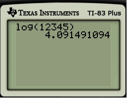
So we estimate $10^{0.9387} \approx 8.684$ This matches the result of a modern calculator to four significant digits:

How to use the table, Part 7.

How to use the table, Part 8.

Note: Sorry, but I’m not sure what happened… when the post came up this morning (August 4), I saw my work in Parts 7 and 8 had disappeared. Maybe one of these days I’ll restore this.

Square roots and logarithms without a calculator (Part 3)

Today’s topic is the use of log tables. I’m guessing that many readers have either forgotten how to use a log table or else were never even taught how to use them. After showing how log tables were used in the past, I’ll conclude with some thoughts about its effectiveness for teaching students logarithms for the first time.

This will be a fairly long post about log tables. In the next post, I’ll discuss how log tables can be used to compute square roots.

To begin, let’s again go back to a time before the advent of pocket calculators… say, 1912.

Before the advent of pocket calculators, most professional scientists and engineers had mathematical tables for keeping the values of logarithms, trigonometric functions, and the like. The following images come from one of my prized possessions: College Mathematics, by Kaj L. Nielsen (Barnes & Noble, New York, 1958). Some saint gave this book to me as a child in the late 1970s; trust me, it was well-worn by the time I actually got to college.

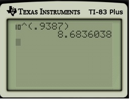
With the advent of cheap pocket calculators, mathematical tables are a relic of the past. The only place that any kind of mathematical table common appears in modern use are in statistics textbooks for providing areas and critical values of the normal distribution, the Student $t$ distribution, and the like.

That said, mathematical tables are not a relic of the remote past. When I was learning logarithms and trigonometric functions at school in the early 1980s — one generation ago — I distinctly remember that my school textbook had these tables in the back of the book.

And it’s my firm opinion that, as an exercise in history, log tables can still be used today to deepen students’ facility with logarithms. In this post and Part 4 of this series, I discuss how the log table can be used to compute logarithms and (using the language of past generations) antilogarithms without a calculator. In Part 5, I’ll discuss my opinions about the pedagogical usefulness of log tables, even if logarithms can be computed more easily nowadays with scientific calculators. In Part 6, I’ll return to square roots — specifically, how log tables can be used to find square roots.

How to use the table, Part 1. How do you read this table? The left-most column shows the ones digit and the tenths digit, while the top row shows the hundredths digit. So, for example, the bottom row shows ten different base-10 logarithms:

$\log_{10} 9.90 \approx 0.9956, \log_{10} 9.91 \approx 0.9961, \log_{10} 9.92 \approx 0.9965,$

$\log_{10} 9.93 \approx 0.9969, \log_{10} 9.94 \approx 0.9974, \log_{10} 9.95 \approx 0.9978,$

$\log_{10} 9.96 \approx 0.9983, \log_{10} 9.97 \approx 0.9987, \log_{10} 9.98 \approx 0.9991,$

$\log_{10} 9.99 \approx 0.9996$

So, rather than punching numbers into a calculator, the table was used to find these logarithms. You’ll notice that these values match, to four decimal places, the values found on a modern calculator.

How to use the table, Part 2. What if we’re trying to take the logarithm of a number between $1$ and $10$ which has more than two digits after the decimal point, like $\log_{10} 5.1264$ ? From the table, we know that the value has to lie between

$\log_{10} 5.12 \approx 0.7093$ and $\log_{10} 5.13 \approx 0.7101$

So, to estimate $\log_{10} 5.1264$ , we will employ linear interpolation. That’s a fancy way of saying “Find the line connecting $(5.12,0.7093)$ and $(5.13,0.7101)$ , and find the point on the line whose $x-$ coordinate is $5.1264$ . The graph of $y = \log_{10} x$ is not a straight line, of course, but hopefully this linear interpolation will be reasonably close to the correct answer.

Finding this line is a straightforward exercise in the point-slope form of a line:

$m = \displaystyle \frac{0.7101-0.7093}{5.13-5.12} = 0.08$

$y - 0.7093= 0.08 (x - 5.12)$

$y = 0.7093+ 0.08 (5.1264-5.12)$

$y = 0.7093+ 0.08(0.0064) = 0.7093 + 0.000512 = 0.709812$

Remembering that this log table is only good to four significant digits, we estimate $\log_{10} 5.1264 \approx 0.7098$ .

Again, this matches the result of a modern calculator to four decimal places:

How to use the table, Part 3. So far, we’ve discussed taking the logarithms of numbers between $1$ and $10$ and the antilogarithms of numbers between $0$ and $1$ . Let’s now consider what happens if we pick a number outside of these intervals.

To find $\log_{10} 12,345$ , we observe that

$\log_{10}12345 = \log_{10} (10,000 \times 1.2345)$

$\log_{10} 12345 = \log_{10} 10,000 + \log_{10} 1.2345$

$\log_{10} 12345 = 4 + \log_{10} 1.2345$

More intuitively, we know that the answer must lie between $\log_{10} 10,000 = 4$ and $100,000 = 5$ , so the answer must be $4.\hbox{something}$ . The value of $\log_{10} 1.2345$ is the necessary $\hbox{something}$ .

We then find $\log_{10} 1.2345$ by linear interpolation. From the table, we see that

$\log_{10} 1.23 \approx 0.0899$ and $\log_{10} 1.24 \approx 0.0934$

Employing linear interpolation, we find

$m = \displaystyle \frac{0.0934-0.0899}{1.24-1.23} = 0.35$

$y - 0.0899= 0.35 (x - 1.23)$

$y = 0.0899+ 0.35 (1.2345-1.23)$

$y = 0.0899+ 0.35(0.0045) = 0.0899 + 0.001575 = 0.091475$

Remembering that this log table is only good to four significant digits, we estimate $\log_{10} 1.2345 \approx 0.0915$ , so that $\log_{10} 12,345 \approx 4.0915$ .

Again, this matches the result of a modern calculator to four decimal places (in this case, five significant digits):

How to use the table, Part 4. Let’s now consider what happens if we pick a positive number less than $1$ . To find $\log_{10} 0.00012345$ , we observe that

$\log_{10}0.00012345 = \log_{10} \left( 1.2345 \times 10^{-4} \right)$

$\log_{10}0.00012345 = \log_{10} 1.2345 + \log_{10} 10^{-4}$

$\log_{10} 0.00012345 = -4 + \log_{10} 1.2345$

We have already found $\log_{10} 1.2345 \approx 0.0915$ by linear interpolation. We therefore conclude that $\log_{10} 12,345 \approx 0.0915 - 4 = -3.9085$ . Again, this matches the result of a modern calculator to four decimal places (in this case, five significant digits):

So that’s how to compute logarithms without a calculator: we rely on somebody else’s hard work to compute these logarithms (which were found in the back of every precalculus textbook a generation ago), and we make clever use of the laws of logarithms and linear interpolation.

Log tables are of course subject to roundoff errors. (For that matter, so are pocket calculators, but the roundoff happens so deep in the decimal expansion — the 12th or 13th digit — that students hardly ever notice the roundoff error and thus can develop the unfortunate habit of thinking that the result of a calculator is always exactly correct.)

For a two-page table found in a student’s textbook, the results were typically accurate to four significant digits. Professional engineers and scientists, however, needed more accuracy than that, and so they had entire books of tables. A table showing 5 places of accuracy would require about 20 printed pages, while a table showing 6 places of accuracy requires about 200 printed pages. Indeed, if you go to the old and dusty books of any decent university library, you should be able to find these old books of mathematical tables.

In other words, that’s how the Brooklyn Bridge got built in an era before pocket calculators.

At this point you may be asking, “OK, I don’t need to use a calculator to use a log table. But let’s back up a step. How were the values in the log table computed without a calculator?” That’s a perfectly reasonable question, but this post is getting long enough as it is. Perhaps I’ll address this issue in a future post.

Advertising for slide rules, from 1940

I’m about to begin a series of posts concerning how previous generations did complex mathematical calculations without the aid of scientific calculators.

Courtesy of Slide Rule Universe, here’s an advertisement for slide rules from 1940. This is a favorite engagement activity of mine when teaching precalculus (as an application of logarithms) as well as my capstone class for future high school math teachers. I have shown this to hundreds of college students over the years (usually reading out loud the advertising through page 5 and then skimming through the remaining pictures), and this always gets a great laugh. Enjoy.

test

Height

I’m about to do a series of posts concerning square roots and logarithms. So I thought that this picture would be an appropriate introduction to the topic. (One of these days, I’ll spring for the wall poster version of this picture to hang in my office.)

Source: http://www.xkcd.com/482/