In this series of posts, I explore properties of complex numbers that explain some surprising answers to exponential and logarithmic problems using a calculator (see video at the bottom of this post). These posts form the basis for a sequence of lectures given to my future secondary teachers.
To begin, we recall that the trigonometric form of a complex number  is
is

where  and
and  , with
  in the appropriate quadrant. As noted before, this is analogous to converting from rectangular coordinates to polar coordinates.
Over the past few posts, we developed the following theorem for computing  in the case that
  is a complex number.
Theorem. If  , where
  and
and  are real numbers, then

As a consequence, there are infinitely many complex solutions of the equation
 ,
,
namely,  .
.
Choosing the solution that has an imaginary part in the interval ![(-\pi,\pi]](https://s0.wp.com/latex.php?latex=%28-%5Cpi%2C%5Cpi%5D&bg=ffffff&fg=000000&s=0&c=20201002) leads to the definition of the complex logarithm.
leads to the definition of the complex logarithm.
Definition. Let  be a complex number so that
  . Then we define
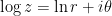 .
.
Of course, this looks like what the definition ought to be if one formally applies the Laws of Logarithms to  . So, for example,
A technicality: this is the principal value of the complex logarithm. In complex analysis, this is technically thought of as a multiply-defined function.
The complex version of the natural logarithm function matches the ordinary definition when applied to real numbers. For example,
 .
.
A couple of observations. In high school, the symbol  is usually dedicated to base 10. However, in higher-level mathematics courses, always means natural logarithm. That’s because, for the purposes of abstract mathematics, base-10 logarithms are practically useless. They are helpful for us people since our number system uses base 10; it’s easy for me to estimate
  , but
, but  requires a little more thought. But nearly all major theorems that involve logarithms specifically employ natural logarithms. Indeed, when I first become a professor, I had to remind myself that my students used
  for natural logarithms and not . Still, I write
  for base-10 logarithms and not as a silent acknowledgment of the use of the symbol in higher-level courses.
This use of the logarithm explains the final results of the calculator in the video below. When  is entered, it assumes that a real answer is expected, and so the calculatore returns an error message. On the other hand, when
  is entered, it assumes that the user wants the principal complex logarithm. Since
  , the calculator correctly returns
  as the answer. (Of course, the calculator still uses and not to mean natural logarithm.)

For completeness, here’s the movie that I use to engage my students when I begin this sequence of lectures.
and
, then
is the inverse function of
.
, we define
.
 . This of course is commonly called the distributive property (and not the commutative property), but the essential idea is that the same answer is obtained whether the multiplications are performed first or if the addition is performed first.
 , then
  .
. .
. .
. .
. is continuous at an interior point
  , then
  .
. are differentiable, then
  .
. .
. .
. .
. is integrable,
  .
. .
. and
and  are random variables, then
  .
. .
. .
. .
. ,
,  , and
, and  are sets, then
  .
. .
. if
if  . Important special cases are
  ,
,  , and
, and  .
. . I call this the
  .
. ,
,  , etc.
 .
. .
.
 .
. .
. .
.
 be complex numbers so that
  . Then we define
 as long as
  , since
  is undefined.
 ,
,  , and
, and  . Then
  .
.![\displaystyle \left[ (-1)^3 \right]^{1/2} \ne (-1)^{3/2}](https://s0.wp.com/latex.php?latex=%5Cdisplaystyle+%5Cleft%5B+%28-1%29%5E3+%5Cright%5D%5E%7B1%2F2%7D+%5Cne+%28-1%29%5E%7B3%2F2%7D&bg=ffffff&fg=000000&s=0&c=20201002) .
. and
and  . Then
  .
. be real numbers and
  .
.![(-2)^{1/2} (-3)^{1/2} \ne \left[ (-2) \cdot (-3) \right]^{1/2}](https://s0.wp.com/latex.php?latex=%28-2%29%5E%7B1%2F2%7D+%28-3%29%5E%7B1%2F2%7D+%5Cne+%5Cleft%5B+%28-2%29+%5Ccdot+%28-3%29+%5Cright%5D%5E%7B1%2F2%7D&bg=ffffff&fg=000000&s=0&c=20201002) .
. that matches De Moivre’s Theorem. Happily, the two definitions agree. Suppose that
  . Then
![= e^{w [\ln r + i \theta]}](https://s0.wp.com/latex.php?latex=%3D+e%5E%7Bw+%5B%5Cln+r+%2B+i+%5Ctheta%5D%7D&bg=ffffff&fg=000000&s=0&c=20201002)


 .
. and
and  and
and  . First,
 .
. .
. . For the base of
  , we note that
 .
. ,
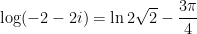
, . To begin,
 .
.


![= e^{-\pi} (\cos [\ln 8] + i \sin [ \ln 8 ] )](https://s0.wp.com/latex.php?latex=%3D+e%5E%7B-%5Cpi%7D+%28%5Ccos+%5B%5Cln+8%5D+%2B+i+%5Csin+%5B+%5Cln+8+%5D+%29&bg=ffffff&fg=000000&s=0&c=20201002)

 , and
, and  .
.
 .
.![\log \left[ (-1) \cdot (-1) \right] = \log 1 = 0](https://s0.wp.com/latex.php?latex=%5Clog+%5Cleft%5B+%28-1%29+%5Ccdot+%28-1%29+%5Cright%5D+%3D+%5Clog+1+%3D+0&bg=ffffff&fg=000000&s=0&c=20201002) ,
, .
.
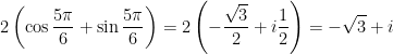
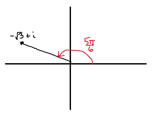
 is in the second quadrant of the complex plane. The modulus is
 .
. , and not
  , so that
 is in the second quadrant, we choose
  . Therefore,
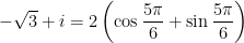
 would also have worked. For example,
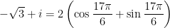

 . After all, the arctangent of an angle must lie between
  and
and  , which won’t work for complex numbers in either the second or third quadrant. That said, it is true that
 , and take two steps to arrive at the point
  , and take two steps to arrive at the same point.
 (getting more than a little dizzy while doing so), and take two steps to arrive at the same point.
 , and take two steps backwards (while doing the moonwalk) to arrive at the same point.
 ? Easy, right? Well, let’s plug into a calculator and find out. (Click anywhere in the image below to start the movie. The important stuff is the screen at the top; you can see the keystrokes that I used if you following the mouse arrow toward the bottom.)