Confirming Einstein’s Theory of General Relativity With Calculus, Part 9: Pedagogical Thoughts

At long last, we have reached the end of this series of posts.

The derivation is elementary; I’m confident that I could have understood this derivation had I seen it when I was in high school. That said, the word “elementary” in mathematics can be a bit loaded — this means that it is based on simple ideas that are perhaps used in a profound and surprising way. Perhaps my favorite quote along these lines was this understated gem from the book Three Pearls of Number Theory after the conclusion of a very complicated proof in Chapter 1:

You see how complicated an entirely elementary construction can sometimes be. And yet this is not an extreme case; in the next chapter you will encounter just as elementary a construction which is considerably more complicated.

Here are the elementary ideas from calculus, precalculus, and high school physics that were used in this series:

Physics
- Conservation of angular momentum
- Newton’s Second Law
- Newton’s Law of Gravitation
Precalculus
- Completing the square
- Quadratic formula
- Factoring polynomials
- Complex roots of polynomials
- Bounds on $\cos \theta$ and $\sin \theta$
- Period of $\cos \theta$ and $\sin \theta$
- Zeroes of $\cos \theta$ and $\sin \theta$
- Trigonometric identities (Pythagorean, sum and difference, double-angle)
- Conic sections
- Graphing in polar coordinates
- Two-dimensional vectors
- Dot products of two-dimensional vectors (especially perpendicular vectors)
- Euler’s equation
Calculus
- The Chain Rule
- Derivatives of $\cos \theta$ and $\sin \theta$
- Linearizations of $\cos x$ , $\sin x$ , and $1/(1-x)$ near $x \approx 0$ (or, more generally, their Taylor series approximations)
- Derivative of $e^x$
- Solving initial-value problems
- Integration by $u-$ substitution

While these ideas from calculus are elementary, they were certainly used in clever and unusual ways throughout the derivation.

I should add that although the derivation was elementary, certain parts of the derivation could be made easier by appealing to standard concepts from differential equations.

One more thought. While this series of post was inspired by a calculation that appeared in an undergraduate physics textbook, I had thought that this series might be worthy of publication in a mathematical journal as an historical example of an important problem that can be solved by elementary tools. Unfortunately for me, Hieu D. Nguyen’s terrific article Rearing Its Ugly Head: The Cosmological Constant and Newton’s Greatest Blunder in The American Mathematical Monthly is already in the record.

Confirming Einstein’s Theory of General Relativity With Calculus, Part 7e: Computing Precession

In this series, I’m discussing how ideas from calculus and precalculus (with a touch of differential equations) can predict the precession in Mercury’s orbit and thus confirm Einstein’s theory of general relativity. The origins of this series came from a class project that I assigned to my Differential Equations students maybe 20 years ago.

We have shown that under general relativity, the motion of a planet around the Sun precesses by

$\phi = \displaystyle \frac{6\pi GM}{ac^2 (1-\epsilon^2)} \qquad \hbox{radians per orbit}$ ,

where $a$ is the semi-major axis of the planet’s orbit, $\epsilon$ is the orbit’s eccentricity, $G$ is the gravitational constant of the universe, $M$ is the mass of the Sun, and $c$ is the speed of light.

Notice that for $\phi$ to be as observable as possible, we’d like $a$ to be as small as possible and $\epsilon$ to be as large as possible. By a fortunate coincidence, the orbit of Mercury — the closest planet to the sun — has the most elliptical orbit of the eight planets.

Here are the values of the constants for Mercury’s orbit in the SI system:

$G = 6.6726 \times 10^{-11} \qquad \hbox{N-m}^2/\hbox{kg}^2$
$M = 1.9929 \times 10^{30} \qquad \hbox{kg}$
$a = 5.7871 \times 10^{10} \qquad \hbox{m}$
$c = 2.9979 \times 10^{8} \qquad \hbox{m/s}$
$\epsilon = 0.2056$
$T = 0.2408 \qquad \hbox{years}$

The last constant, $T$ , is the time for Mercury to complete one orbit. This isn’t in the SI system, but using Earth years as the unit of time will prove useful later in this calculation.

Using these numbers, and recalling that $1 ~ \hbox{N} = 1 ~ \hbox{kg-m/s}^2$ , we find that

$\phi = \displaystyle \frac{6\pi \times 6.6726 \times 10^{-11} ~ \hbox{m}^3/(\hbox{kg-s}^2) \times 1.9929 \times 10^{30} ~ \hbox{kg}}{5.7871 \times 10^{10} ~ \hbox{m} \times (2.9979 \times 10^{8} ~ \hbox{m/s})^2 \times (1-(0.2408)^2)} \approx 5.03 \times 10^{-7}$ .

Notice that all of the units cancel out perfectly; this bit of dimensional analysis is a useful check against careless mistakes.

Again, the units of $\phi$ are in radians per Mercury orbit, or radians per 0.2408 years. We now convert this to arc seconds per century:

$\phi \approx 5.03 \times 10^{-7} \displaystyle \frac{\hbox{radians}}{\hbox{0.2408 years}} \times \frac{180 ~\hbox{degrees}}{\pi ~ \hbox{radians}} \times \frac{3600 ~ \hbox{arc seconds}}{1 ~ \hbox{degree}} \times \frac{100 ~ \hbox{years}}{1 ~ \hbox{century}}$

$\phi = 43.1 \displaystyle \frac{\hbox{arc seconds}}{\hbox{century}}$ .

This indeed matches the observed precession in Mercury’s orbit, thus confirming Einstein’s theory of relativity.

This same computation can be made for other planets. For Venus, we have the new values of $a = 1.0813 \times 10^{11} ~ \hbox{m}$ , $\epsilon = 0.0068$ , and $T = 0.6152 ~ \hbox{years}$ . Repeating this calculation, we predict the precession in Venus’s orbit to be 8.65” per century. Einstein made this prediction in 1915, when the telescopes of the time were not good enough to measure the precession in Venus’s orbit. This only happened in 1960, 45 years later and 5 years after Einstein died. Not surprisingly, the precession in Venus’s orbit also agrees with general relativity.

Confirming Einstein’s Theory of General Relativity With Calculus, Part 7d: Predicting Precession IV

We have shown that the motion of a planet around the Sun, expressed in polar coordinates $(r,theta)$ with the Sun at the origin, under general relativity is

$u(\theta) \approx \displaystyle \frac{1}{\alpha} \left[ 1 + \epsilon \cos \left( \theta - \frac{\delta \theta}{\alpha} \right) \right]$ ,

where $u = \displaystyle \frac{1}{r}$ , $\alpha = a(1-\epsilon^2)$ , $a$ is the semi-major axis of the planet’s orbit, $\epsilon$ is the orbit’s eccentricity, $\delta = \displaystyle \frac{3GM}{c^2}$ , $G$ is the gravitational constant of the universe, $m$ is the mass of the planet, $M$ is the mass of the Sun, $P$ is the planet’s perihelion, $\ell$ is the constant angular momentum of the planet, and $c$ is the speed of light.

The above function $u(\theta)$ is maximized (i.e., the distance from the Sun $r(\theta)$ is minimized) when $\displaystyle \cos \left( \theta - \frac{\delta \theta}{\alpha} \right)$ is as large as possible. This occurs when $\theta - \displaystyle \frac{\delta \theta}{\alpha}$ is a multiple of $2\pi$ .

Said another way, the planet is at its closest point to the Sun when $\theta = 0$ . One orbit later, the planet returns to its closest point to the Sun when

$\theta - \displaystyle \frac{\delta \theta}{\alpha} = 2\pi$

$\theta \displaystyle\left(1 - \frac{\delta}{\alpha} \right) = 2\pi$

$\theta = 2\pi \displaystyle\frac{1}{1 - (\delta/\alpha)}$

We now use the approximation

$\displaystyle \frac{1}{1-x} \approx 1 + x \qquad \hbox{if} \qquad x \approx 0$ ;

this can be demonstrated by linearization, Taylor series, or using the first two terms of the geometric series $1 + x + x^2 + x^3 + \dots$ . With this approximation, the closest approach to the Sun in the next orbit occurs when

$\theta = 2\pi \displaystyle\left(1 + \frac{\delta}{\alpha} \right) = 2\pi + \frac{2\pi \delta}{\alpha}$ ,

which is coterminal with the angle

$\phi = \displaystyle \frac{2\pi \delta}{\alpha}$ .

Substituting $\alpha = a(1-\epsilon^2)$ and $\delta = \displaystyle \frac{3GM}{c^2}$ , we see that the amount of precession per orbit is

$\phi = \displaystyle 2 \pi \frac{3GM}{c^2} \frac{1}{a(1-\epsilon^2)} = \frac{6\pi G M}{ac^2(1-\epsilon^2)}$ .

The units of $\phi$ are radians per orbit. In the next post, we will use Mercury’s data to find $\phi$ in seconds of arc per century.

Confirming Einstein’s Theory of General Relativity With Calculus, Part 7c: Predicting Precession III

We have shown that the motion of a planet around the Sun, expressed in polar coordinates $(r,theta)$ with the Sun at the origin, under general relativity is

$u(\theta) \approx \displaystyle \frac{1}{\alpha} \left[ 1 + \epsilon \cos \left( \theta - \frac{\delta \theta}{\alpha} \right) \right]$ ,

where $u = \displaystyle \frac{1}{r}$ , $\displaystyle \frac{1}{\alpha} = \frac{GMm^2}{\ell^2}$ , $\epsilon = \displaystyle \frac{\alpha - P}{P}$ , $\delta = \displaystyle \frac{3GM}{c^2}$ , $G$ is the gravitational constant of the universe, $m$ is the mass of the planet, $M$ is the mass of the Sun, $P$ is the planet’s perihelion, $\ell$ is the constant angular momentum of the planet, and $c$ is the speed of light.

We notice that the orbit of a planet under general relativity looks very, very similar to the orbit under Newtonian physics:

$u(\theta) \approx \displaystyle \frac{1}{\alpha} \left[ 1 + \epsilon \cos \theta \right]$ ,

so that

$r(\theta) = \displaystyle \frac{\alpha}{1 + \epsilon \cos \theta}$ .

As we’ve seen, this describes an elliptical orbit, normally expressed in rectangular coordinates as

$\displaystyle \frac{(x-h)^2}{a^2} + \frac{y^2}{b^2} = 1$ ,

with semimajor axis along the $x-$ axis. In particular, for an elliptical orbit, the planet’s closest approach to the Sun occurs at $\theta = 0$ :

$r(0) = \displaystyle \frac{\alpha}{1 + \epsilon \cos 0} = \frac{\alpha}{1 + \epsilon}$ ,

and the planet’s further distance from the Sun occurs at $\theta = \pi$ :

$r(\pi) = \displaystyle \frac{\alpha}{1 + \epsilon \cos \pi} = \frac{\alpha}{1 - \epsilon}$ .

Therefore, the length $2a$ of the major axis of the ellipse is the sum of these two distances:

$2a = \displaystyle \frac{\alpha}{1 + \epsilon} + \frac{\alpha}{1 - \epsilon}$

$2a = \displaystyle \frac{\alpha(1-\epsilon) + \alpha(1+\epsilon)}{(1 + \epsilon)(1 - \epsilon)}$

$2a= \displaystyle \frac{2\alpha}{1 - \epsilon^2}$

$a = \displaystyle \frac{\alpha}{1 - \epsilon^2}$ .

Said another way, $\alpha = a(1-\epsilon^2)$ . This is a far more convenient formula for computing $\alpha$ than $\alpha = \displaystyle \frac{\ell^2}{GMm^2}$ , as the values of $a$ (the semi-major axis) and $\epsilon$ (the eccentricity of the orbit) are more accessible than the angular momentum $\ell$ of the planet’s orbit.

In the next post, we finally compute the precession of the orbit.

Confirming Einstein’s Theory of General Relativity With Calculus, Part 7b: Predicting Precession II

We have shown that the motion of a planet around the Sun, expressed in polar coordinates $(r,\theta)$ with the Sun at the origin, under general relativity is

$u(\theta) \approx \displaystyle \frac{1 + \epsilon \cos \theta}{\alpha} + \frac{ \delta\epsilon}{\alpha^2} \theta \sin \theta$ ,

where $u = \displaystyle \frac{1}{r}$ , $\displaystyle \frac{1}{\alpha} = \frac{GMm^2}{\ell^2}$ , $\delta = \displaystyle \frac{3GM}{c^2}$ , $G$ is the gravitational constant of the universe, $m$ is the mass of the planet, $M$ is the mass of the Sun, $\ell$ is the constant angular momentum of the planet, and $c$ is the speed of light.

We will now simplify this expression, using the facts that $\delta$ is very small and $\alpha$ is quite large, so that $\delta/\alpha$ is very small indeed. We will use the two approximations

$\cos x \approx 1 \qquad \hbox{and} \qquad \sin x \approx x \qquad \hbox{if} \qquad x \approx 0$ ;

these approximations can be obtained by linearization or else using the first term of the Taylor series expansions of $\cos x$ and $\sin x$ about $x = 0$ .

We will also need the trig identity

$\cos(\theta_1 - \theta_2) = \cos \theta_1 \cos \theta_2 + \sin \theta_1 \sin \theta_2$ .

With these tools, we can now simplify $u(\theta)$ :

$u(\theta) \approx \displaystyle \frac{1 + \epsilon \cos \theta}{\alpha} + \frac{ \delta\epsilon}{\alpha^2} \theta \sin \theta$

$= \displaystyle \frac{1}{\alpha} \left[1 + \epsilon \cos \theta + \frac{ \delta\epsilon}{\alpha} \theta \sin \theta \right]$

$= \displaystyle \frac{1}{\alpha} \left[1 + \epsilon \left(\cos \theta + \frac{ \delta}{\alpha} \theta \sin \theta \right) \right]$

$= \displaystyle \frac{1}{\alpha} \left[1 + \epsilon \left(\cos \theta \cdot 1 + \sin \theta \cdot \frac{ \delta \theta}{\alpha} \right) \right]$

$\approx \displaystyle \frac{1}{\alpha} \left[1 + \epsilon \left(\cos \theta \cdot \cos \frac{\delta \theta}{\alpha} + \sin \theta \cdot \sin \frac{ \delta \theta}{\alpha} \right) \right]$

$\approx \displaystyle \frac{1}{\alpha} \left[1 + \epsilon \cos \left( \theta - \frac{\delta \theta}{\alpha} \right) \right]$ .

Square roots and logarithms without a calculator (Part 10)

This is the fifth in a series of posts about calculating roots without a calculator, with special consideration to how these tales can engage students more deeply with the secondary mathematics curriculum. As most students today have a hard time believing that square roots can be computed without a calculator, hopefully giving them some appreciation for their elders.

Today’s story takes us back to a time before the advent of cheap pocket calculators: 1949.

The following story comes from the chapter “Lucky Numbers” of Surely You’re Joking, Mr. Feynman!, a collection of tales by the late Nobel Prize winning physicist, Richard P. Feynman. Feynman was arguably the greatest American-born physicist — the subject of the excellent biography Genius: The Life and Science of Richard Feynman — and he had a tendency to one-up anyone who tried to one-up him. (He was also a serial philanderer, but that’s another story.) Here’s a story involving how, in the summer of 1949, he calculated $\sqrt[3]{1729.03}$ without a calculator.

The first time I was in Brazil I was eating a noon meal at I don’t know what time — I was always in the restaurants at the wrong time — and I was the only customer in the place. I was eating rice with steak (which I loved), and there were about four waiters standing around.

A Japanese man came into the restaurant. I had seen him before, wandering around; he was trying to sell abacuses. (Note: At the time of this story, before the advent of pocket calculators, the abacus was arguably the world’s most powerful hand-held computational device.) He started to talk to the waiters, and challenged them: He said he could add numbers faster than any of them could do.

The waiters didn’t want to lose face, so they said, “Yeah, yeah. Why don’t you go over and challenge the customer over there?”

The man came over. I protested, “But I don’t speak Portuguese well!”

The waiters laughed. “The numbers are easy,” they said.

They brought me a paper and pencil.

The man asked a waiter to call out some numbers to add. He beat me hollow, because while I was writing the numbers down, he was already adding them as he went along.

I suggested that the waiter write down two identical lists of numbers and hand them to us at the same time. It didn’t make much difference. He still beat me by quite a bit.

However, the man got a little bit excited: he wanted to prove himself some more. “Multiplição!” he said.

Somebody wrote down a problem. He beat me again, but not by much, because I’m pretty good at products.

The man then made a mistake: he proposed we go on to division. What he didn’t realize was, the harder the problem, the better chance I had.

We both did a long division problem. It was a tie.

This bothered the hell out of the Japanese man, because he was apparently well trained on the abacus, and here he was almost beaten by this customer in a restaurant.

“Raios cubicos!” he says with a vengeance. Cube roots! He wants to do cube roots by arithmetic. It’s hard to find a more difficult fundamental problem in arithmetic. It must have been his topnotch exercise in abacus-land.

He writes down a number on some paper— any old number— and I still remember it: $1729.03$ . He starts working on it, mumbling and grumbling: “Mmmmmmagmmmmbrrr”— he’s working like a demon! He’s poring away, doing this cube root.

Meanwhile I’m just sitting there.

One of the waiters says, “What are you doing?”.

I point to my head. “Thinking!” I say. I write down $12$ on the paper. After a little while I’ve got $12.002$ .

The man with the abacus wipes the sweat off his forehead: “Twelve!” he says.

“Oh, no!” I say. “More digits! More digits!” I know that in taking a cube root by arithmetic, each new digit is even more work that the one before. It’s a hard job.

He buries himself again, grunting “Rrrrgrrrrmmmmmm …,” while I add on two more digits. He finally lifts his head to say, “ $12.0$ !”

The waiter are all excited and happy. They tell the man, “Look! He does it only by thinking, and you need an abacus! He’s got more digits!”

He was completely washed out, and left, humiliated. The waiters congratulated each other.

How did the customer beat the abacus?

The number was $1729.03$ . I happened to know that a cubic foot contains $1728$ cubic inches, so the answer is a tiny bit more than $12$ . The excess, $1.03$ , is only one part in nearly $2000$ , and I had learned in calculus that for small fractions, the cube root’s excess is one-third of the number’s excess. So all I had to do is find the fraction $1/1728$ , and multiply by $4$ (divide by $3$ and multiply by $12$ ). So I was able to pull out a whole lot of digits that way.

A few weeks later, the man came into the cocktail lounge of the hotel I was staying at. He recognized me and came over. “Tell me,” he said, “how were you able to do that cube-root problem so fast?”

I started to explain that it was an approximate method, and had to do with the percentage of error. “Suppose you had given me $28$ . Now the cube root of $27$ is $3$ …”

He picks up his abacus: zzzzzzzzzzzzzzz— “Oh yes,” he says.

I realized something: he doesn’t know numbers. With the abacus, you don’t have to memorize a lot of arithmetic combinations; all you have to do is to learn to push the little beads up and down. You don’t have to memorize 9+7=16; you just know that when you add 9, you push a ten’s bead up and pull a one’s bead down. So we’re slower at basic arithmetic, but we know numbers.

Furthermore, the whole idea of an approximate method was beyond him, even though a cubic root often cannot be computed exactly by any method. So I never could teach him how I did cube roots or explain how lucky I was that he happened to choose $1729.03$ .

The key part of the story, “for small fractions, the cube root’s excess is one-third of the number’s excess,” deserves some elaboration, especially since this computational trick isn’t often taught in those terms anymore. If $f(x) = (1+x)^n$ , then $f'(x) = n (1+x)^{n-1}$ , so that $f'(0) = n$ . Since $f(0) = 1$ , the equation of the tangent line to $f(x)$ at $x = 0$ is

$L(x) = f(0) + f'(0) \cdot (x-0) = 1 + nx$ .

The key observation is that, for $x \approx 0$ , the graph of $L(x)$ will be very close indeed to the graph of $f(x)$ . In Calculus I, this is sometimes called the linearization of $f$ at $x =a$ . In Calculus II, we observe that these are the first two terms in the Taylor series expansion of $f$ about $x = a$ .

For Feynman’s problem, $n =\frac{1}{3}$ , so that $\sqrt[3]{1+x} \approx 1 + \frac{1}{3} x$ if $x \approx 0$. Then $\latex \sqrt[3]{1729.03}$ can be rewritten as

$\sqrt[3]{1729.03} = \sqrt[3]{1728} \sqrt[3]{ \displaystyle \frac{1729.03}{1728} }$

$\sqrt[3]{1729.03} = 12 \sqrt[3]{\displaystyle 1 + \frac{1.03}{1728}}$

$\sqrt[3]{1729.03} \approx 12 \left( 1 + \displaystyle \frac{1}{3} \times \frac{1.03}{1728} \right)$

$\sqrt[3]{1729.03} \approx 12 + 4 \times \displaystyle \frac{1.03}{1728}$

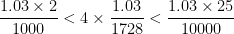
This last equation explains the line “all I had to do is find the fraction $1/1728$ , and multiply by $4$ .” With enough patience, the first few digits of the correction can be mentally computed since

$\displaystyle \frac{1.03}{500} < \frac{1.03}{432} = 4 \times \frac{1.03}{1728} < \frac{1.03}{400}$

$\displaystyle \frac{1.03 \times 2}{1000} < 4 \times \frac{1.03}{1728} < \frac{1.03 \times 25}{10000}$

$0.00206 < 4 \times \displaystyle \frac{1.03}{1728} < 0.0025075$

So Feynman could determine quickly that the answer was $12.002\hbox{something}$ .

By the way,

$\sqrt[3]{1729.03} \approx 12.00238378\dots$

$\hbox{Estimate} \approx 12.00238426\dots$

So the linearization provides an estimate accurate to eight significant digits. Additional digits could be obtained by using the next term in the Taylor series.

I have a similar story to tell. Back in 1996 or 1997, when I first moved to Texas and was making new friends, I quickly discovered that one way to get odd facial expressions out of strangers was by mentioning that I was a math professor. Occasionally, however, someone would test me to see if I really was a math professor. One guy (who is now a good friend; later, we played in the infield together on our church-league softball team) asked me to figure out $\sqrt{97}$ without a calculator — before someone could walk to the next room and return with the calculator. After two seconds of panic, I realized that I was really lucky that he happened to pick a number close to $100$ . Using the same logic as above,

$\sqrt{97} = \sqrt{100} \sqrt{1 - 0.03} \approx 10 \left(1 - \displaystyle \frac{0.03}{2}\right) = 9.85$ .

Knowing that this came from a linearization and that the tangent line to $y = \sqrt{1+x}$ lies above the curve, I knew that this estimate was too high. But I didn’t have time to work out a correction (besides, I couldn’t remember the full Taylor series off the top of my head), so I answered/guessed $9.849$ , hoping that I did the arithmetic correctly. You can imagine the amazement when someone punched into the calculator to get $9.84886\dots$