The following problem appeared in Volume 97, Issue 3 (2024) of Mathematics Magazine.
Two points and are chosen at random (uniformly) from the interior of a unit circle. What is the probability that the circle whose diameter is segment lies entirely in the interior of the unit circle?
As discussed in a previous post, I guessed from simulation that the answer is . Naturally, simulation is not a proof, and so I started thinking about how to prove this.
My first thought was to make the problem simpler by letting only one point be chosen at random instead of two. Suppose that the point is fixed at a distance from the origin. What is the probability that the point , chosen at random, uniformly, from the interior of the unit circle, has the desired property?
My second thought is that, by radial symmetry, I could rotate the figure so that the point is located at . In this way, the probability in question is ultimately going to be a function of .
There is a very nice way to compute such probabilities since is chosen at uniformly from the unit circle. Let be the set of all points within the unit circle that have the desired property. Since the area of the unit circle is , the probability of desired property happening is
.
Based on the simulations discussed in the previous post, my guess was that was the interior of an ellipse centered at the origin with a semimajor axis of length and a semiminor axis of length . Now I had to think about how to prove this.
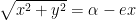
As noted earlier in this series, the circle with diameter will lie within the unit circle exactly when , where is the midpoint of . So suppose that has coordinates , where is known, and let the coordinates of be . Then the coordinates of will be
,
so that
and
.
Therefore, the condition (again, equivalent to the condition that the circle with diameter lies within the unit circle) becomes
,
which simplifies to
.
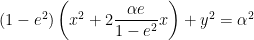
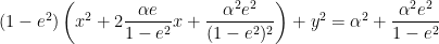
When I saw this, light finally dawned. Given two points and , called the foci, an ellipse is defined to be the set of all points so that , where is a constant. If the coordinates of , , and are , , and , then this becomes
.
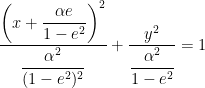
Therefore, the set is the interior of an ellipse centered at the origin with and . Furthermore, is the semimajor axis of the ellipse, while the semiminor axis is equal to .
At last, I could now return to the original question. Suppose that the point is fixed at a distance from the origin. What is the probability that the point , chosen at random, uniformly, from the interior of the unit circle, has the property that the circle with diameter lies within the unit circle? Since is a subset of the interior of the unit circle, we see that this probability is equal to
.
In the next post, I’ll use this intermediate step to solve the original question.
At long last, we have reached the end of this series of posts.
The derivation is elementary; I’m confident that I could have understood this derivation had I seen it when I was in high school. That said, the word “elementary” in mathematics can be a bit loaded — this means that it is based on simple ideas that are perhaps used in a profound and surprising way. Perhaps my favorite quote along these lines was this understated gem from the book Three Pearls of Number Theory after the conclusion of a very complicated proof in Chapter 1:
You see how complicated an entirely elementary construction can sometimes be. And yet this is not an extreme case; in the next chapter you will encounter just as elementary a construction which is considerably more complicated.
Here are the elementary ideas from calculus, precalculus, and high school physics that were used in this series:
Physics
Conservation of angular momentum
Newton’s Second Law
Newton’s Law of Gravitation
Precalculus
Completing the square
Quadratic formula
Factoring polynomials
Complex roots of polynomials
Bounds on and
Period of and
Zeroes of and
Trigonometric identities (Pythagorean, sum and difference, double-angle)
Conic sections
Graphing in polar coordinates
Two-dimensional vectors
Dot products of two-dimensional vectors (especially perpendicular vectors)
Euler’s equation
Calculus
The Chain Rule
Derivatives of and
Linearizations of , , and near (or, more generally, their Taylor series approximations)
Derivative of
Solving initial-value problems
Integration by substitution
While these ideas from calculus are elementary, they were certainly used in clever and unusual ways throughout the derivation.
I should add that although the derivation was elementary, certain parts of the derivation could be made easier by appealing to standard concepts from differential equations.
One more thought. While this series of post was inspired by a calculation that appeared in an undergraduate physics textbook, I had thought that this series might be worthy of publication in a mathematical journal as an historical example of an important problem that can be solved by elementary tools. Unfortunately for me, Hieu D. Nguyen’s terrific article Rearing Its Ugly Head: The Cosmological Constant and Newton’s Greatest Blunder in The American Mathematical Monthly is already in the record.
In this series, I’m discussing how ideas from calculus and precalculus (with a touch of differential equations) can predict the precession in Mercury’s orbit and thus confirm Einstein’s theory of general relativity. The origins of this series came from a class project that I assigned to my Differential Equations students maybe 20 years ago.
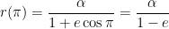
We have shown that the motion of a planet around the Sun, expressed in polar coordinates with the Sun at the origin, under general relativity is
,
where , , , , is the gravitational constant of the universe, is the mass of the planet, is the mass of the Sun, is the planet’s perihelion, is the constant angular momentum of the planet, and is the speed of light.
We notice that the orbit of a planet under general relativity looks very, very similar to the orbit under Newtonian physics:
,
so that
.
As we’ve seen, this describes an elliptical orbit, normally expressed in rectangular coordinates as
,
with semimajor axis along the axis. In particular, for an elliptical orbit, the planet’s closest approach to the Sun occurs at :
,
and the planet’s further distance from the Sun occurs at :
.
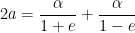
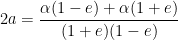
Therefore, the length of the major axis of the ellipse is the sum of these two distances:
.
Said another way, . This is a far more convenient formula for computing than , as the values of (the semi-major axis) and (the eccentricity of the orbit) are more accessible than the angular momentum of the planet’s orbit.
In the next post, we finally compute the precession of the orbit.
In this series, I’m discussing how ideas from calculus and precalculus (with a touch of differential equations) can predict the precession in Mercury’s orbit and thus confirm Einstein’s theory of general relativity. The origins of this series came from a class project that I assigned to my Differential Equations students maybe 20 years ago.
As part of our derivation, we’ll need to use the fact that, in polar coordinates, the graph of
turns out to be an ellipse if , with the origin at one focus.
We now prove this. Clearing the denominator, we obtain
.
Switching to rectangular coordinates, this becomes
Since we assumed that , we have so that
.
Therefore, this matches the usual form of an ellipse in rectangular coordinates
,
where the center of the ellipse is located at
,
the semi-major axis is horizontal with length
,
and the semi-minor axis is vertical with length
.
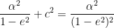
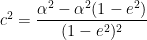
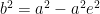
Furthermore, the distance of the foci from the center of the ellipse satisfies the equation
,
so that
From this, we derive two nice properties of the ellipse. First, looking back on previous work, we see that . Therefore, since the foci of the ellipse are distance away from the center along the major axis, we conclude that one focus of the ellipse is located at , or . That is, the origin is one focus of the ellipse. (For the little it’s worth, the other focus is located at .
Second, the eccentricity of the ellipse is defined to be the ratio . This is now easily computed:
.
In other words, the letter was well-chosen to represent the eccentricity of the ellipse.
For what it’s worth, here’s an alternate derivation of the formulas for and . For this ellipse, the planet’s closest approach to the Sun occurs at :
,
and the planet’s further distance from the Sun occurs at :
.
Therefore, the length of the major axis of the ellipse is the sum of these two distances:
In this series, I’m discussing how ideas from calculus and precalculus (with a touch of differential equations) can predict the precession in Mercury’s orbit and thus confirm Einstein’s theory of general relativity. The origins of this series came from a class project that I assigned to my Differential Equations students maybe 20 years ago.
But what is precession? To explore this concept, let’s explore the graph of
for various values of , , and using Desmos. (Note that, in this context, the number does not mean Euler’s constant . The reason for choosing the letter for this parameter will become clear shortly.) Naturally, this demonstration could also be done with other tools like a graphing calculator.
I suggest beginning by setting and and altering the value of . This is the easiest behavior to explain. From the equation, is directly proportional to the distance from the origin . So, not surprisingly, increasing produces a larger graph, and decreasing produces a smaller graph.
Second, I suggest setting and but altering the value of . Starting at , the graph is a circle. This makes complete sense: if , then the equation simply becomes , so the distance from the origin is the same for all angles. However, as increases, the original circle becomes more and more stretched out. We will prove this analytically in a later post, but it turns out that, for , the graph is an ellipse, and the origin is one of the foci of the ellipse. The number is called the eccentricity of the ellipse (hence the letter ).
Again, if the value of is fixed but varies, the graph becomes either larger or smaller as becomes larger or smaller.
We notice that if and , then the denominator of
varies between and . In particular, the denominator is always positive. Therefore, the value of is least positive — the graph is closest to the origin — when the denominator is greatest. This happens when is a multiple of . So, for example, when , then is as close as the graph gets to the origin. Let’s call this closest distance ; in the context of a planet’s orbit around the sun, this represent perihelion. Then we have .
When , the graph switches from an ellipse to a parabola, where the origin is the focus of the parabola. For , the graph becomes a hyperbola. However, since we’re mostly going to be concerned with stable planetary orbits in this series, we won’t dwell too much on the case .
Third, I suggest setting , , and then alter the value of . For , the graph is simply a single ellipse. However, by changing the value of , the graph changes into a spiral.
In the above figure, the spiral stopped “spiraling” because I had asked Desmos only to show the graph between . If I had changed the upper bound to something larger than , the spiral would continue.
The precession in the spiral is defined to be the angular offset between each loop of the spiral. Clearly, this is a function of . To find this function, we again examine the function
Once again, if , then the denominator varies between and . In particular, the denominator is always positive. Therefore, the value of is least positive when the denominator is greatest, and the denominator is greatest when is a multiple of . So, for example, when , then is as close as the graph gets to the origin.
When does the graph return to its closest point to the origin next? This would occur when , or . If , then the angle of closest approach to the origin would , and the graph simply cycles over itself. However, if , then this angle will be larger than , thus producing a spiral. Indeed, the amount of precession would be equal to
.
In the picture above, . Therefore, the amount of precession would be radians . Therefore, after 19 “leafs” of the spiral, the graph would begin to cycle on top of itself.
In this series, I’m discussing how ideas from calculus and precalculus (with a touch of differential equations) can predict the precession in Mercury’s orbit and thus confirm Einstein’s theory of general relativity. The origins of this series came from a class project that I assigned to my Differential Equations students maybe 20 years ago.
This is going to be a very long series, so I’d like to provide a tree-top view of how the argument will unfold.
We begin by using three principles from Newtonian physics — the Law of Conservation of Angular Momentum, Newton’s Second Law, and Newton’s Law of Gravitation — to show that the orbit of a planet, under Newtonian physics, satisfies the initial-value problem
,
,
.
In these equations:
The orbit of the planet is in polar coordinates , where the Sun is placed at the origin.
The planet’s perihelion — closest distance from the Sun — is a distance of at angle .
The function is equal to .
is the gravitational constant of the universe.
is the mass of the Sun.
is the mass of the planet.
is the angular momentum of the planet.
The solution of this differential equation is
,
so that
.
In polar coordinates, this is the graph of an ellipse. Substituting , we see that
.
In the solution for , we have and . The number is the eccentricity of the ellipse, while is proportional to the size of the ellipse.
Under general relativity, the governing initial-value problem changes to
,
,
,
where is the speed of light. We will see that the solution of this new differential equation can be well approximated by
.
This last equation describes a spiral that precesses by approximately
radians per orbit
or
radians per orbit,
where is the length of the semimajor axis of the orbit.
This matches the amount of precession in Mercury’s orbit that is not explained by Newtonian physics, thus confirming Einstein’s theory of general relativity.
To the extent possible, I will take the perspective of a good student who has taken Precalculus and Calculus I. However, I will have to break this perspective a couple of times when I discuss principles from physics and derive the solutions of the above differential equations.
In this series, I’m discussing how ideas from calculus and precalculus (with a touch of differential equations) can predict the precession in Mercury’s orbit and thus confirm Einstein’s theory of general relativity. The origins of this series came from a class project that I assigned to my Differential Equations students maybe 20 years ago.
The figure below shows the (greatly exaggerated) effect of precession on a planet’s otherwise elliptical orbit. In the figure, each perihelion is precessed by an angle of . After nine orbits, the planet returns to its original position. Suppose, for the sake of argument, that each orbit of the planet depicted in the figure is four months, or one third of Earth’s year. Then the amount of precession would be per four months, or per year, or per century.
As I said, the figure above is greatly exaggerated. As we’ll see by the end of this series, Einstein’s general relativity predicts that, on top of the gravitational influences of the other planets, the orbit of Mercury should precess by 43″ of arc per century. That’s a really small angle, since 1 is equal to 60′ (minutes) of arc and each 1′ is equal to 60″ (seconds) of arc, that means 1″ of arc is the same as , so that 43″ of arc per century is about per century. That’s about a million times smaller than the precession of the fictitious planet in the above figure.
How small is , really?
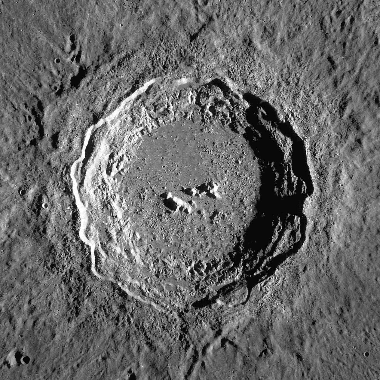
Courtesy of Wikipedia, the pictures below are the Copernicus crater on the Moon as well as an indicator of its location on the Moon. It is visible with binoculars.
The diameter of the crater is 93 km. Since the Moon is 384,400 km from Earth, that means the angle subtended by the crater, as viewed from the Earth, is about
.
So how much is 43″ of arc per century? That’s about the speed as, hypothetically, pointing at the left edge of this lunar crater (which cannot be seen by the naked eye) and then slowly moving your figure so that, about 115 years later, your finger is pointing at the right edge of the crater.
Said another way, the diameter of the Moon is about 3475 km, so that the angle subtended by the Moon, as viewed from the Earth, is about
.
So, at the rate of per century, it would take centuries, or about 43,000 years, to trace the angle subtended by the moon.
Needless to say, 43” of arc per century is really, really slow.
Nevertheless, and remarkably, this itty, bitty precession was observable by careful 19th century astronomers with the telescopes that were available then. At the time, this precession was the great unsolved mystery of Newtonian physics that was only answered after two generations later with the discovery of general relativity.
If the universe consisted of only Mercury and the sun, Mercury’s trajectory would trace the same ellipse over and over again. However, there are seven other planets in the solar system (not to mention the dwarf planets), and these planets tug and nudge the orbit of Mercury ever so slightly. (For what it’s worth, similar nudges in the orbit of Uranus led to the discovery of Neptune in 1846.)
The practical effect of these nudges is that the orbit of Mercury precesses, or rotates like a spiral. The figure below shows the (greatly exaggerated) effect of precession on a planet’s otherwise elliptical orbit. In the figure, each perihelion is precessed by an angle of . After nine orbits, the planet returns to its original position.
Since the planets are much smaller than the sun and are further away from the Sun than Mercury, this precession is very small. However, this effect can be measured. Every century, the perihelion of Mercury precesses by 574” of arc (roughly a sixth of a degree).
Newton’s Law of Gravitation can be used to calculate the amount of the precession of Mercury; however, they predict a precession of only 531” of arc per century. This discrepancy between observation and prediction was first observed in 1845 and was, for a long time, the outstanding unresolved difficulty in Newtonian physics.
Einstein’s general theory of relativity, which was published seventy years later in 1915, exactly accounts for the missing 43” per century (within the tolerances of observational error). This was the first physical confirmation of general relativity. Furthermore, general relativity predicted that the orbit of Venus also precesses, but by only about 9” of arc per century. This small discrepancy was unobservable in 1915 but was confirmed in 1960. (While not logically necessary, that’s certainly indicative of an accurate scientific theory… not that it merely explains the world but it makes a prediction that is currently unobservable.)
In this series, which might take me a few months to complete, I’m going to explore how to predict the precession in Mercury’s orbit — i.e., confirm Einstein’s theory of general relativity — using tools only from calculus and precalculus. I first introduced these ideas as a class project for my Differential Equations students maybe 20 years ago. As we’ll see, in a couple spots, ideas from first-semester differential equations can make the steps more rigorous. However, pretty much this whole series should be accessible to a good calculus student.
I should say at the outset that none of the mathematics in this series is particularly original with me. I gladly acknowledge that I first learned the ideas in this series as an undergraduate, when I took an upper-level physics course in mechanics. In particular, pretty much all of the ideas in this series can be found in the textbook Classical Dynamics of Particles and Systems, by S. T. Thornton and J. B. Marion (Brooks Cole, New York, 2003). If I’ve made any contribution, it’s the scaffolding of these ideas to make them accessible to students who won’t be taking (or haven’t yet taken) physics courses beyond the traditional first-year sequence.
The proofs of Kepler’s Three Laws are usually included in textbooks for multivariable calculus. So I was very intrigued when I saw, in the Media Reviews of College Mathematics Journal, that somebody had published a proof of Kepler’s First Law that only uses algebra and trigonometry. Let me quote from the review:
Kepler’s first law states that bounded planetary orbits are elliptical. This law is presented in introductory textbooks, but the proof typically requires intricate integrals or vector analysis involving an accidental degeneracy. Simha offers an elementary proof of Kepler’s first law using algebra and trigonometry at the high school level.
Once upon a time, I taught Precalculus for precocious high school students. I wish I had known of this result back then, as it would have been a wonderful capstone to their studies of trigonometry and the conic sections.
The preprint of this result can be found on arXiv. (The proof only addresses Kepler’s First Law and not the Second and Third Laws.) The actual article, for those with institutional access, was published in American Journal of Physics Vol. 89 No. 11 (2021): 1009-1011.
In my capstone class for future secondary math teachers, I ask my students to come up with ideas for engaging their students with different topics in the secondary mathematics curriculum. In other words, the point of the assignment was not to devise a full-blown lesson plan on this topic. Instead, I asked my students to think about three different ways of getting their students interested in the topic in the first place.
I plan to share some of the best of these ideas on this blog (after asking my students’ permission, of course).
This student submission comes from my former student Peter Buhler. His topic, from Precalculus: graphing an ellipse.
How could you as a teacher create an activity or project that involves your topic?
One project that could be assigned to students during the unit on conic sections could be to challenge students to either find or make an ellipse. This could be with a household object, a computer simulated object, or it could be something such as the movement of the planets around the sun. Students would be expected to visually display their object(s) of choice, as well as provide an equation for the ellipse. For example, if the student chose to use a deflated basketball or football, students would use the actual units found when measuring the object and then create an equation for that ellipse. Of course, students would also be expected to graph the ellipse using the appropriate equation, and then check the graph with the actual object (if possible). This project would allow students to be creative in choosing something of ellipse form, and would allow them to further explore the graphing and equation-building of an ellipse.
How can this topic be used in your students’ future courses in mathematics or science?
While graphing an ellipse is a topic within the Pre-Calculus curriculum, it also has applications within other topics as well. One of these is the unit circle, which is also taught in most Pre-Calculus courses. The unit circle is simply an ellipse where both major and minor axis are of length 1, as well as the center at (0,0). Students can be encouraged to draw comparisons between the two topics. Not only can they rewrite the equation of an ellipse to fit the unit circle, but students can also use the distance formula to calculate sine and cosine values on the unit circle. They can then use the distance formula on various forms of an ellipse, and compare and contrast between the two.
Later on in a students’ mathematical career, some students may encounter ellipse used in three dimensions in Calculus III, in an engineering course, or even in an astronomy course. Ellipses have many applications, and students may benefit from you (as the teacher) perhaps mentioning some of these applications when going over the unit on conic sections.
How has this topic appeared in high culture?
One particularly intriguing application of an ellipse (among many applications) is in the design of a whispering gallery. This is essentially a piece of architecture that is designed in the shape of an ellipse so that when someone is standing at one focus of the ellipse, they can clearly hear someone whispering from the exact location of the other focus. Some of examples of these “whispering rooms include St. Paul’s Cathedral, the Echo Wall in Beijing, and in the U.S. Capitol building. It has been commonly noted that President John Quincy Adams would eavesdrop on others while standing in the Capitol, simply due to the physics of sound waves traveling inside an ellipse shaped building.
On a more personal business, I can remember multiple visits to the Science Museum in Fair Park, where various forms of sciences were displayed in formats that children (and adults!) could interact with. There was one exhibit that was set up for several years that also incorporated this ellipse-shaped architecture. I remember it clearly, due to the fact that I was so fascinated with how I could stand 30 yards from someone and be able to hear their whisper clearly. This could also be a class project or even a class trip that would allow students to hypothesize why this works the way it does. It can be noted that this would work for both Physics and Math classes, as it has applications to both.
and
are chosen at random (uniformly) from the interior of a unit circle. What is the probability that the circle whose diameter is segment
lies entirely in the interior of the unit circle?


![\displaystyle \sqrt{ \frac{1}{4} \left[ (x+t)^2 + y^2 \right]} + \sqrt{ \frac{1}{4} \left[ (x-t)^2 + y^2 \right]} < 1](https://s0.wp.com/latex.php?latex=%5Cdisplaystyle+%5Csqrt%7B+%5Cfrac%7B1%7D%7B4%7D+%5Cleft%5B+%28x%2Bt%29%5E2+%2B+y%5E2+%5Cright%5D%7D+%2B+%5Csqrt%7B+%5Cfrac%7B1%7D%7B4%7D+%5Cleft%5B+%28x-t%29%5E2+%2B+y%5E2+%5Cright%5D%7D+%3C+1&bg=ffffff&fg=000000&s=0&c=20201002)


 and
and 
 ,
,  , and
, and  near
near  (or, more generally, their Taylor series approximations)
 substitution
 with the Sun at the origin, under general relativity is
 ![u(\theta) \approx \displaystyle \frac{1}{\alpha} \left[ 1 + \epsilon \cos \left( \theta - \frac{\delta \theta}{\alpha} \right) \right]](https://s0.wp.com/latex.php?latex=u%28%5Ctheta%29+%5Capprox++%5Cdisplaystyle+%5Cfrac%7B1%7D%7B%5Calpha%7D+%5Cleft%5B+1+%2B+%5Cepsilon+%5Ccos+%5Cleft%28+%5Ctheta+-+%5Cfrac%7B%5Cdelta+%5Ctheta%7D%7B%5Calpha%7D+%5Cright%29+%5Cright%5D&bg=ffffff&fg=000000&s=0&c=20201002) ,
, ,
,  ,
,  ,
,  ,
,  is the gravitational constant of the universe,
  is the mass of the planet,
  is the constant angular momentum of the planet, and
  is the speed of light.
![u(\theta) \approx \displaystyle \frac{1}{\alpha} \left[ 1 + \epsilon \cos \theta \right]](https://s0.wp.com/latex.php?latex=u%28%5Ctheta%29+%5Capprox++%5Cdisplaystyle+%5Cfrac%7B1%7D%7B%5Calpha%7D+%5Cleft%5B+1+%2B+%5Cepsilon+%5Ccos+%5Ctheta+%5Cright%5D&bg=ffffff&fg=000000&s=0&c=20201002) ,
, .
. ,
, axis. In particular, for an elliptical orbit, the planet’s closest approach to the Sun occurs at
  :
: ,
, :
: .
. of the major axis of the ellipse is the sum of these two distances:


 .
. . This is a far more convenient formula for computing
  than
than  , as the values of
  (the eccentricity of the orbit) are more accessible than the angular momentum
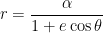
 , with the origin at one focus.
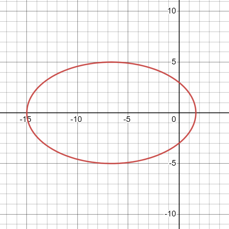
 .
.


 so that
 .
. ,
, ,
, ,
, .
. ,
,


 . Therefore, since the foci of the ellipse are distance
  , or
, or  . That is, the origin is one focus of the ellipse. (For the little it’s worth, the other focus is located at
  .
. . This is now easily computed:
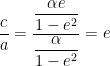 .
. was well-chosen to represent the eccentricity of the ellipse.
 . For this ellipse, the planet’s closest approach to the Sun occurs at
 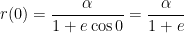 ,
, .
.

 .
. , we can also compute


 using
using  . The reason for choosing the letter
  and
and  and altering the value of
  . So, not surprisingly, increasing
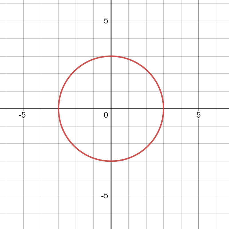
 and
and  , so the distance from the origin is the same for all angles. However, as
 and
and  . In particular, the denominator is always positive. Therefore, the value of
  is a multiple of
  . So, for example, when
  is as close as the graph gets to the origin. Let’s call this closest distance
  .
. , the graph switches from an ellipse to a parabola, where the origin is the focus of the parabola. For
  , the graph becomes a hyperbola. However, since we’re mostly going to be concerned with stable planetary orbits in this series, we won’t dwell too much on the case
  .
. , and then alter the value of
 . If I had changed the upper bound to something larger than
  , the spiral would continue.
 is a multiple of
  , or
, or  . If
. If  , then the angle of closest approach to the origin would
  , and the graph simply cycles over itself. However, if
  , then this angle
  .
. . Therefore, the amount of precession would be
  radians
  . Therefore, after 19 “leafs” of the spiral, the graph would begin to cycle on top of itself.
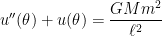 ,
, ,
, .
. , where the Sun is placed at the origin.
 is equal to
  .
. ,
, .
. is proportional to the size of the ellipse.
![u''(\theta) + u(\theta) = \displaystyle \frac{GMm^2}{\ell^2} + \frac{3GM}{c^2} [u(\theta)]^2](https://s0.wp.com/latex.php?latex=u%27%27%28%5Ctheta%29+%2B+u%28%5Ctheta%29+%3D+%5Cdisplaystyle+%5Cfrac%7BGMm%5E2%7D%7B%5Cell%5E2%7D+%2B+%5Cfrac%7B3GM%7D%7Bc%5E2%7D+%5Bu%28%5Ctheta%29%5D%5E2&bg=ffffff&fg=000000&s=0&c=20201002) ,
,
![\approx \displaystyle \frac{1}{\alpha} \left[1 + \epsilon \cos \left(\theta - \frac{\delta \theta}{\alpha} \right) \right]](https://s0.wp.com/latex.php?latex=%5Capprox+%5Cdisplaystyle+%5Cfrac%7B1%7D%7B%5Calpha%7D+%5Cleft%5B1+%2B+%5Cepsilon+%5Ccos+%5Cleft%28%5Ctheta+-+%5Cfrac%7B%5Cdelta+%5Ctheta%7D%7B%5Calpha%7D+%5Cright%29+%5Cright%5D&bg=ffffff&fg=000000&s=0&c=20201002) .
. radians per orbit
 radians per orbit,
 . After nine orbits, the planet returns to its original position. Suppose, for the sake of argument, that each orbit of the planet depicted in the figure is four months, or one third of Earth’s year. Then the amount of precession would be
  per four months, or
  per year, or
  per century.
 is equal to 60′ (minutes) of arc and each 1′ is equal to 60″ (seconds) of arc, that means 1″ of arc is the same as
  , so that 43″ of arc per century is about
  per century. That’s about a million times smaller than the precession of the fictitious planet in the above figure.
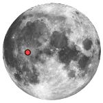
 .
. .
. centuries, or about 43,000 years, to trace the angle subtended by the moon.