Different definitions of logarithm (Part 7)

There are two apparently different definitions of a logarithm that appear in the secondary mathematics curriculum:

From Algebra II and Precalculus: If $a > 0$ and $a \ne 1$ , then $f(x) = \log_a x$ is the inverse function of $g(x) = a^x$ .
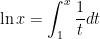
From Calculus: for $x > 0$ , we define $\ln x = \displaystyle \int_1^x \frac{1}{t} dt$ .

The connection between these two apparently different ideas begins with the following theorem, which was proven in the few previous posts.

Theorem. Let $a \in \mathbb{R}^+ \setminus \{1\}$ . Suppose that $f: \mathbb{R}^+ \rightarrow \mathbb{R}$ has the following four properties:

$f(1) = 0$

$f(a) = 1$

$f(xy) = f(x) + f(y)$ for all $x, y \in \mathbb{R}^+$

$f$ is continuous

Then $f(x) = \log_a x$ for all $x \in \mathbb{R}^+$ .

At this point, we have provided enough groundwork to make the connection between these two different ways of viewing a logarithm.

Let’s define the function (for $x > 0$ )

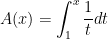
$A(x) = \displaystyle \int_1^x \frac{1}{t} dt$ .

I’ll illustrate this with the appropriate area under the hyperbola $y = \frac{1}{x}$ . (Please forgive the crudeness of this drawing; I’m only using Microsoft Paint.)

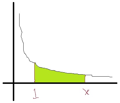
So if $x$ is the right-hand limit, then $A(x)$ is just the shaded area under the curve.

Often, someone will interject, “Hey, I know how to do that… it’s just the natural logarithm of $x$ .” To which I will respond, “Yes, that’s true. But why is it the natural logarithm of $x$ ?” I have yet to encounter a student who can immediately answer this question (which, of course, is the whole point of me presenting this in class). In other words, I want my students to realize that, many semesters ago, they pretty much accepted on faith that the above integral is equal to $\ln x$ , but they were never told the reason why. And now — several semesters after completing the calculus sequence — we’re finally going over the reason why.

To start, I’ll say, “OK, $A$ is defined as an integral. That means that it must have…” Someone will usually volunteer, “A derivative.” I’ll respond, “That’s right. The Fundamental Theorem of Calculus says that this function is differentiable. So, if something is differentiable, then it also must be…” Someone will usually volunteer, “Continuous.” My response: “That’s right. So $A$ must be continuous. So that’s Property 4: this function is continuous.” I’ll continue: “Let’s see if we can get the other properties.”

I’ll next move to Property 1, as it’s the next easiest. I’ll ask the class, “Can you prove to me that $A(1) = 0$ ?” After a moment of thought, someone will notice that

$A(1) = \displaystyle \int_1^1 \frac{1}{t} dt$ .

must be equal to $0$ since the left and right endpoints of the integral are the same.

Then I’ll skip over to Property 3, which requires a little more thought. To begin, we can write

$A(xy) = \displaystyle \int_1^{xy} \frac{1}{t} dt = \displaystyle \int_1^{x} \frac{1}{t} dt + \int_x^{xy} \frac{1}{t} dt$ .

Before proceeding, I’ll ask my class why the above line has to be true. After a couple moments, someone will volunteer something like “The area from $1$ to $x$ plus the area from $x$ to $xy$ has to be equal to the area from $1$ to $xy$ .”

I’ll then say something like, “We can simplify one of the integrals on the right-hand side right away. Which one?” Students quickly see that the first integral on the right, $\displaystyle \int_1^{x} \frac{1}{t} dt$ , is of course equal to $A(x)$ . So then I’ll ask, “So what do I want the last integral to be equal to?” Students look back at Property 3 and answer, “That should be $A(y)$ .

So, if we can show the final integral is equal to $A(y)$ , we have established Property 3. To this end, I will perform a somewhat unusual looking $u-$ substitution:

$t = ux$

In this formula, I encourage my students to think of $t$ as the old variable of integration, $u$ as the new variable of integration, and $x$ as an unknown number that is constant. So I’ll say parenthetically, “If $t = 5u$ , how do we find $dt$ ?” Students of course answer, “ $dt$ must be $5 du$ .” So I’ll follow up: “If $t = xu$ , how do we find $dt$ ?” Students get the idea:

$t = x \, du$

So to complete the $u-$ substitution, we must adjust the limits of integration. For the lower limit,

$t = x \Longrightarrow u = \displaystyle \frac{x}{x} = 1$

For the upper limit,

$t = xy \Longrightarrow u = \displaystyle \frac{xy}{x} = y$

So we can now complete the $u-$ substitution of the second integral:

$A(xy) = \displaystyle \int_1^{xy} \frac{1}{t} dt = \displaystyle \int_1^{x} \frac{1}{t} dt + \int_x^{xy} \frac{1}{t} dt$ .

$A(xy) = \displaystyle \int_1^{x} \frac{1}{t} dt + \int_1^{y} \frac{1}{xu} x \, du$ .

$A(xy) = \displaystyle \int_1^{x} \frac{1}{t} dt + \int_1^{y} \frac{1}{u} \, du$ .

Students recognize that, except for the variable of integration, the last integral is just $A(y)$ , which leads to the punch line

$A(xy) = A(x) + A(y)$

In other words, we have established that the function $A$ satisfies Property 3.

So the only property left is Property 2. To that end, let’s define the number $e$ so that the area in green above is equal to 1. There’s no other way to describe this number…. we just increase $x$ far enough along the $x-$ axis until the area under the hyperbola is equal to 1. Wherever this happens, that’s the number that we’ll call $e$ . So, by definition, $A(e) = 1$ .

Therefore, by the above theorem, we conclude that $A(x) = \log_e x$ , written more simply as $\ln x$ .

To summarize: using the above theorem, we are able to establish that the integral $\displaystyle \int_1^x \frac{1}{t} dt$ has all of the properties of a logarithm and therefore must be a logarithmic function. The only catch is that we had to define $e$ to be the base of this logarithm through an unusual definition concerning the area under a hyperbola.

Of course, this is not the “standard” definition of $e$ that is usually encountered in a Precalculus class. More on these different definitions in a future series of posts.

One more pedagogical note: My experience is that I can cover the content of the first 7 posts of this series in a single 50-minute lecture and still keep my students’ attention. Naturally, I’ll recapitulate the highlights of this logical development at the start of the next lecture by way of review, as this is an awful lot to absorb at once.

Different definitions of logarithm (Part 6)

There are two apparently different definitions of a logarithm that appear in the secondary mathematics curriculum:

From Algebra II and Precalculus: If $a > 0$ and $a \ne 1$ , then $f(x) = \log_a x$ is the inverse function of $g(x) = a^x$ .
From Calculus: for $x > 0$ , we define $\ln x = \displaystyle \int_1^x \frac{1}{t} dt$ .

The connection between these two apparently different ideas begins with the following theorem.

Theorem. Let $a \in \mathbb{R}^+ \setminus \{1\}$ . Suppose that $f: \mathbb{R}^+ \rightarrow \mathbb{R}$ has the following four properties:

$f(1) = 0$

$f(a) = 1$

$f(xy) = f(x) + f(y)$ for all $x, y \in \mathbb{R}^+$

$f$ is continuous

Then $f(x) = \log_a x$ for all $x \in \mathbb{R}^+$ .

Note. To prove this theorem, I will show that $f(a^x) = x$ , thus proving that $f$ is the inverse of $g(x) = a^x$ .

The proof of these theorem divides into four cases:

Positive integers: $x = m \in \mathbb{Z}^+$
Positive rational numbers: $x = \frac{m}{n}$ , where $m,n \in \mathbb{Z}^+$
Negative rational numbers: $x \in \mathbb{Q}^-$
Real (possibly irrational) numbers: $x \in \mathbb{R}$

In today’s post, I’ll complete the proof by handling Case 4.

Before starting Case 4, I like to take inventory of where we stand in the proof at this point. We have now proven the theorem for all positive rational numbers and for all negative rational numbers. There’s only one rational number left: $x = 0$ . And this single case is simply handled through Property 1:

$f(a^0) = f(1) = 0$

I also like to keep track of which hypotheses have been used so far in the proof. A quick review of Cases 1-3 will reveal that Properties 1-3 have all been used at least once, but Property 4 (the assumption that $f$ is continuous) has not be used so far. Therefore, we had better expect to use it before completing the proof.

I won’t tell the class this (for fear of discouraging them), but the proof of Case 4 is a bit more abstract than Cases 1-3. I can give a numerical example that (hopefully) will shed some insight into the actual proof. However, for Case 4, the actual proof will not be a perfect parallel of the numerical example (as in Cases 1-3).

Idea behind Case 4. Let’s pick a familiar irrational number like $\sqrt{2}$ . There is a natural way to approximate $\sqrt{2}$ by a sequence of rational numbers… namely, the sequence of numbers obtained by taking one extra digit in the decimal expansion of $\sqrt{2}$ . In other words,

$r_1 = 1$

$r_2 = 1.4$

$r_3 = 1.41$

$r_4 = 1.414$

and so on.

In this way, $\displaystyle \lim_{n \to \infty} r_n = \sqrt{2}$ .

We would hope that the sequence

$f \left( a^1 \right), f \left( a^{1.4} \right), f \left( a^{1.41} \right), f \left( a^{1.414} \right), \dots$

converges to the obvious limit of

$f \left( a^{\sqrt{2}} \right)$ .

However, this sequence is also equal to

$1, 1.4, 1.41, 1.414, \dots$

since each exponent is rational. Since a sequence has only one limit, we conclude that these two limits should be equal:

$\sqrt{2} = f \left( a^{\sqrt{2}} \right)$

So that’s the idea of the formal proof, which we now tackle. In the proof below, I’ve marked with quotations some of the more parenthetical steps so that the main argument of the proof stands out a little bit better. You’ll notice that, unlike Cases 1-3, I don’t use as much directed questioning to get students to volunteer the next step of the proof with minimal assistance from me. That’s because I haven’t figured out a good way to use inquiry to quickly get through Case 4.

Proof of Case 4. Let $\{ r_n \}$ be a sequence of rational numbers that converges to $x$ . (Parenthetically, I’ll mention that the sequence of decimal approximations would be one such sequence, just to make this mysterious $\{ r_n \}$ thing that just appeared out of the blue a little less daunting. Of course, any sequence of rational numbers that converges to $x$ will do. Therefore,

$f \left( a^x \right) = f \left( a^{\lim_{n \to \infty} r_n} \right)$

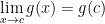
The function $g(x) = a^x$ is continuous. From the ordinary definition of continuous used in calculus, this means that

$\displaystyle \lim_{x \to c} g(x) = g(c)$ .

In other words, the function and the limit can be interchanged. (I’ll usually throw in my standard joke about functions commuting at this point in the lecture.) Stated in terms of a sequence $r_n \to x$ , this means that

$\displaystyle \lim_{n \to \infty} g(r_n) = g(x) = g \left( \lim_{n \to \infty} r_n \right)$ .

Stated another way,

$\displaystyle \lim_{n \to \infty} a^{r_n} = a^{ \lim_{n \to \infty} r_n}$ .

In light of the above work, we conclude that

$f \left( a^x \right) = f \left( a^{\lim_{n \to \infty} r_n} \right) = f \left( \displaystyle \lim_{n \to \infty} a^{r_n} \right)$

Stated simply, the function and the limit interchange.

We now perform a similar step for the function $f$ . Because $f$ is assumed to be continuous, we know that

$\displaystyle \lim_{n \to \infty} f(s_n) = f(c) = f \left( \lim_{n \to \infty} s_n \right)$

if $\{ s_n \}$ is a sequence that converges to $c$ . So, if we replace $s_n$ by $a^{r_n}$ and $c$ by $\displaystyle \lim_{n \to \infty} a^{r_n}$ , we conclude that

$\displaystyle \lim_{n \to \infty} f \left( a^{r_n} \right) = f \left( \displaystyle \lim_{n \to \infty} a^{r_n} \right)$

From the above insight, we see that we have the next step of the proof:

$f \left( a^x \right) = f \left( a^{\lim_{n \to \infty} r_n} \right)$

$= f \left( \displaystyle \lim_{n \to \infty} a^{r_n} \right)$

$= \displaystyle \lim_{n \to \infty} f \left(a^{r_n} \right)$

From now on, the concluding steps are pretty straightforward. The exponent on the last line is a rational number. Therefore, by Cases 2 and 3, we have produce the next step:

$f \left( a^x \right) = f \left( a^{\lim_{n \to \infty} r_n} \right)$

$= f \left( \displaystyle \lim_{n \to \infty} a^{r_n} \right)$

$= \displaystyle \lim_{n \to \infty} f \left(a^{r_n} \right)$

$= \displaystyle \lim_{n \to \infty} r_n$

Finally, by definition from the top of the proof, we can evaluate this limit:

$f \left( a^x \right) = f \left( a^{\lim_{n \to \infty} r_n} \right)$

$= f \left( \displaystyle \lim_{n \to \infty} a^{r_n} \right)$

$= \displaystyle \lim_{n \to \infty} f \left(a^{r_n} \right)$

$= \displaystyle \lim_{n \to \infty} r_n$

$= x$

This concludes the proof that $f \left( a^x \right) = x$ , even if $x$ is an arbitrary (possibly irrational) real number.

Different definitions of logarithm (Part 5)

There are two apparently different definitions of a logarithm that appear in the secondary mathematics curriculum:

From Algebra II and Precalculus: If $a > 0$ and $a \ne 1$ , then $f(x) = \log_a x$ is the inverse function of $g(x) = a^x$ .
From Calculus: for $x > 0$ , we define $\ln x = \displaystyle \int_1^x \frac{1}{t} dt$ .

The connection between these two apparently different ideas begins with the following theorem.

Theorem. Let $a \in \mathbb{R}^+ \setminus \{1\}$ . Suppose that $f: \mathbb{R}^+ \rightarrow \mathbb{R}$ has the following four properties:

$f(1) = 0$

$f(a) = 1$

$f(xy) = f(x) + f(y)$ for all $x, y \in \mathbb{R}^+$

$f$ is continuous

Then $f(x) = \log_a x$ for all $x \in \mathbb{R}^+$ .

Note. To prove this theorem, I will show that $f(a^x) = x$ , thus proving that $f$ is the inverse of $g(x) = a^x$ .

The proof of these theorem divides into four cases:

Positive integers: $x = m \in \mathbb{Z}^+$
Positive rational numbers: $x = \frac{m}{n}$ , where $m,n \in \mathbb{Z}^+$
Negative rational numbers: $x \in \mathbb{Q}^-$
Real (possibly irrational) numbers: $x \in \mathbb{R}$

In today’s post, I’ll describe how I prompt my students to prove Case 3 during class time. Cases 4 will appear in tomorrow’s post.

Idea behind Case 3. Though not formally necessary for the proof, I’ve found it helpful to illustrate the idea of the proof with a specific example before proceeding to the general case. So — on the far end of the chalkboard, away from the space that I’ve allocated for the formal write-up of the proof — I’ll write

$f \left( a^{-2/3} \cdot a^{2/3} \right) =$

I’ll then ask, “How else can we simplify the left-hand side?” As we’ll see below, there are actually two legitimate ways of proceeding. Someone will usually suggest just simplifying the product, and so I’ll write this as the next step:

$f \left( a^{-2/3} \cdot a^{2/3} \right) = f \left( a^0 \right)$

I’ll then ask a very open-ended question, “Now what?” Usually, someone will suggest simplifying the right-hand side using Property 1:

$f \left( a^{-2/3} \cdot a^{2/3} \right) = f \left( a^0 \right) = 0$

By this point, after completing Cases 1 and 2, someone will usually suggest expanding the left-hand side:

$f \left( a^{-2/3} \right) + f \left( a^{2/3} \right) = 0$

I’ll then ask, “What can we do now?” Hopefully, someone will observe that the second term can be simplified using Case 2:

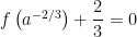
$f \left( a^{-2/3} \right) + \displaystyle \frac{2}{3} = 0$

$f \left( a^{-2/3} \right) = - \displaystyle \frac{2}{3}$

I’ll then note that we’ve finished what we set out to do: show that $f(a^x) = x$ when $x = - \frac{2}{3}$ , a negative rational number.

The natural next question is, “Can we do this for any negative rational number and not just $-\frac{2}{3}$ ?” This leads to the proof of Case 3. I’ve found that it’s helpful to walk through this proof line by line in step with the case of $x= -\frac{2}{3}$ , so that students can see how the steps of this more abstract proof correspond to the concrete example of $x = =\frac{2}{3}$ .

Proof of Case 3. Let $m, n \in \mathbb{Z}^+$ . Then

$f \left(a^{-m/n} \cdot a^{m/n} \right) = f \left(a^0 \right)$

$f \left( a^{-m/n} \right) + f \left( a^{m/n} \right) = 0$

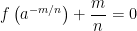
$f \left( a^{-m/n} \right) + \displaystyle \frac{m}{n} = 0$

$f \left( a^{-m/n} \right) = - \displaystyle \frac{m}{n}$

Again, I’ve found that the special case $x = - \frac{2}{3}$ is pedagogically helpful, if not logically necessary to prove Case 3.

Different definitions of logarithm (Part 4)

There are two apparently different definitions of a logarithm that appear in the secondary mathematics curriculum:

From Algebra II and Precalculus: If $a > 0$ and $a \ne 1$ , then $f(x) = \log_a x$ is the inverse function of $g(x) = a^x$ .
From Calculus: for $x > 0$ , we define $\ln x = \displaystyle \int_1^x \frac{1}{t} dt$ .

The connection between these two apparently different ideas begins with the following theorem.

Theorem. Let $a \in \mathbb{R}^+ \setminus \{1\}$ . Suppose that $f: \mathbb{R}^+ \rightarrow \mathbb{R}$ has the following four properties:

$f(1) = 0$

$f(a) = 1$

$f(xy) = f(x) + f(y)$ for all $x, y \in \mathbb{R}^+$

$f$ is continuous

Then $f(x) = \log_a x$ for all $x \in \mathbb{R}^+$ .

Note. To prove this theorem, I will show that $f(a^x) = x$ , thus proving that $f$ is the inverse of $g(x) = a^x$ .

The proof of these theorem divides into four cases:

Positive integers: $x = m \in \mathbb{Z}^+$
Positive rational numbers: $x = \frac{m}{n}$ , where $m,n \in \mathbb{Z}^+$
Negative rational numbers: $x \in \mathbb{Q}^-$
Real (possibly irrational) numbers: $x \in \mathbb{R}$

In today’s post, I’ll describe how I prompt my students to prove Case 2 during class time. Cases 3-4 will appear in the coming posts.

Idea behind Case 2. Though not formally necessary for the proof, I’ve found it helpful to illustrate the idea of the proof with a specific example before proceeding to the general case. So — on the far end of the chalkboard, away from the space that I’ve allocated for the formal write-up of the proof — I’ll write

$2 = f(a^2)$

I’ll ask, “How do we know this is true?” The immediate answer: We just did Case 1. I’ll then do something a little unusual and rewrite this equation in a more complicated way:

$2 = f(a^2) = f \left( \left[a^{2/3} \right]^3 \right)$

After double-checking that the class agrees with this step (even if I just made the right-hand more complicated instead of the usual step of simplifying the right-hand side), I’ll then ask, “OK, we have something to the third power. What can we now do to the right-hand side?” Almost immediately, someone will volunteer the correct next steps using Property 3:

$2 = f(a^2) = f \left( a^{2/3} \cdot a^{2/3} \cdot a^{2/3} \right) = f \left( a^{2/3} \right) + f \left( a^{2/3} \right) + f \left( a^{2/3} \right)$

I’ll then ask, “How can we simplify the right-hand side?” After a moment of thought, someone will volunteer the correct next step:

$2 = f(a^2) = f \left( a^{2/3} \cdot a^{2/3} \cdot a^{2/3} \right) = f \left( a^{2/3} \right) + f \left( a^{2/3} \right) + f \left( a^{2/3} \right)$

$2 = 3 f \left( a^{2/3} \right)$

I’ll then ask, “How do we isolate the $f \left( a^{2/3} \right)$ term?” The obvious correct answer:

$\displaystyle \frac{2}{3} = f(a^{2/3})$

I’ll then note that we’ve finished what we set out to do: show that $f(a^x) = x$ when $x = \frac{2}{3}$ .

The natural next question is, “Can we do this for any positive rational number and not just $\frac{2}{3}$ ?” This leads to the proof of Case 2. I’ve found that it’s helpful to walk through this proof line by line in step with the case of $x=\frac{2}{3}$ , so that students can see how the steps of this more abstract proof correspond to the concrete example of $x =\frac{2}{3}$ .

Proof of Case 2. Let $x = \displaystyle \frac{m}{n}$ where $m, n \in \mathbb{R}^+$ . Then

$m = f(a^m)$

$m = f \left( \left[ a^{m/n} \right]^n \right)$

$m = f \left( a^{m/n} \cdot a^{m/n} \cdot \dots \cdot a^{m/n} \right)$

$m = f \left( a^{m/n} \right) + f \left( a^{m/n} \right) + \dots + f \left( a^{m/n} \right)$

$m = n f \left( a^{m/n} \right)$

$\displaystyle \frac{m}{n} = f \left( a^{m/n} \right)$

Of course, the special case $x = \frac{2}{3}$ is not logically necessary to prove Case 2. Though not logically necessary, I’ve found it to be pedagogically convenient. From the school of hard knocks, I’ve found that the proof of Case 2 goes over easier with students when they see the idea of the proof presented concretely and then abstractly.

Different definitions of logarithm (Part 3)

There are two apparently different definitions of a logarithm that appear in the secondary mathematics curriculum:

From Algebra II and Precalculus: If $a > 0$ and $a \ne 1$ , then $f(x) = \log_a x$ is the inverse function of $g(x) = a^x$ .
From Calculus: for $x > 0$ , we define $\ln x = \displaystyle \int_1^x \frac{1}{t} dt$ .

The connection between these two apparently different ideas begins with the following theorem.

Theorem. Let $a \in \mathbb{R}^+ \setminus \{1\}$ . Suppose that $f: \mathbb{R}^+ \rightarrow \mathbb{R}$ has the following four properties:

$f(1) = 0$

$f(a) = 1$

$f(xy) = f(x) + f(y)$ for all $x, y \in \mathbb{R}^+$

$f$ is continuous

Then $f(x) = \log_a x$ for all $x \in \mathbb{R}^+$ .

Note. To prove this theorem, I will show that $f(a^x) = x$ , thus proving that $f$ is the inverse of $g(x) = a^x$ .

The proof of these theorem divides into four cases:

Positive integers: $x = m \in \mathbb{Z}^+$
Positive rational numbers: $x = \frac{m}{n}$ , where $m,n \in \mathbb{Z}^+$
Negative rational numbers: $x \in \mathbb{Q}^-$
Real (possibly irrational) numbers: $x \in \mathbb{R}$

In today’s post, I’ll describe how I prompt my students to prove Case 1 during class time. Cases 2-4 will appear in the coming posts.

Idea behind Case 1. Though not formally necessary for the proof, I’ve found it helpful to illustrate the idea of the proof with a specific example before proceeding to the general case. So — on the far end of the chalkboard, away from the space that I’ve allocated for the formal write-up of the proof — I’ll write

$f(a^4) =$

I’ll then ask, “How else can we write $a^4$ ?” Someone will usually suggest $a \cdot a \cdot a \cdot a$ , and so I’ll write this as the next step:

$f(a^4) = f(a \cdot a \cdot a \cdot a)$

I’ll then ask, “OK, we have a product here. How can we simplify the right-hand side?” After a moment of thought, someone will volunteer that Property 3 allows the right-hand side to be split up into pieces:

$f(a^4) = f(a \cdot a \cdot a \cdot a) = f(a) + f(a) + f(a) + f(a)$

(Technically, this requires mathematical induction to generalize Property 3 from a product of two numbers to a product of arbitrarily many numbers, but I don’t think that it’s worth the time to expound on this pedantic point.) I’ll then ask, “How can we simplify this?” Almost immediately, someone will usually volunteer Property 2:

$f(a^4) = f(a \cdot a \cdot a \cdot a) = f(a) + f(a) + f(a) + f(a) = 1 + 1 + 1 + 1 = 4$

I’ll then note that we’ve finished what we set out to do: show that $f(a^x) = x$ when $x = 4$ .

The natural next question is, “Can we do this for any positive integer and not just 4?” This leads to the proof of Case 1. I’ve found that it’s helpful to walk through this proof line by line in step with the case of $x=4$ , so that students can see how the steps of this more abstract proof correspond to the concrete example of $x =4$ .

Proof of Case 1.

$f(a^m) = f(a \cdot a \cdot \dots \cdot a)$

$= f(a) + f(a) + \dots + f(a)$

$= 1 + 1 + \dots + 1$

$= m$

Of course, the special case $x = 4$ is not logically necessary to prove Case 1. That said, from the school of hard knocks, I’ve found that the proof of Case 1 goes over easier with students when they see the idea of the proof presented concretely and then abstractly.

Different definitions of logarithm (Part 2)

There are two apparently different definitions of a logarithm that appear in the secondary mathematics curriculum:

From Algebra II and Precalculus: If $b > 0$ and $b \ne 1$ , then $f(x) = \log_b x$ is the inverse function of $g(x) = b^x$ .
From Calculus: for $x > 0$ , we define $\ln x = \displaystyle \int_1^x \frac{1}{t} dt$ .

In this series of posts, we examine the interrelationship between these two different approaches to logarithms. This is a standard topic in my class for future teachers of secondary mathematics as a way of deepening their understanding of a topic that they think they know quite well.

The connection between these two apparently different ideas begins with the following theorem.

Theorem. Let $a \in \mathbb{R}^+ \setminus \{1\}$ . Suppose that $f: \mathbb{R}^+ \rightarrow \mathbb{R}$ has the following four properties:

$f(1) = 0$

$f(a) = 1$

$f(xy) = f(x) + f(y)$ for all $x, y \in \mathbb{R}^+$

$f$ is continuous

Then $f(x) = \underline{\hspace{1in}}$ for all $x \in \mathbb{R}^+$ .

When writing this on the board, I purposefully leave an underline for my students to fill in, because I want them to think. What familiar function has these four properties? I’ll usually invoke the old chidren’s joke: “If it looks like an elephant, smells like an elephant, feels like an elephant, and sounds like an elephant, then it must be an elephant.” After a moment of thought, someone will usually volunteer $f(x) = \log x$ . That’s almost correct, and so I’ll ask if Property 2 is satisfied by this function. After a couple more moments of thought, someone will volunteer the correct answer, $f(x) = \log_a x$ .

To prove this theorem, I will show that

$f(a^x) = x$ for all $x \in \mathbb{R}$ .

I’ll make the observation that the case of $latex x=0$ is Property 1, while the case of $x = 1$ is Property 2.

Then I’ll ask the class: “If I’m able to prove that $f(a^x) = x$ for all real $x$ , why does this mean that $f(x) = \log_a x$ ?” Perhaps unsurprisingly, this usually draws blank stares for a few seconds until someone realizes that this means that $f: \mathbb{R}^+ \rightarrow \mathbb{R}$ and $g: \mathbb{R} \rightarrow \mathbb{R}^+$ defined by $g(x) = a^x$ are inverse functions. So (by definition) $f(x)$ must be equal to $\log_a x$ .

The proof of these theorem has four parts:

Positive integers: $x = m \in \mathbb{Z}^+$
Positive rational numbers: $x = \frac{m}{n}$ , where $m,n \in \mathbb{Z}^+$
Negative rational numbers: $x \in \mathbb{Q}^-$
Real (possibly irrational) numbers: $x \in \mathbb{R}$

Beginning with tomorrow’s post, I’ll discuss how I walk students through the proof in lecture.

Different definitions of logarithm (Part 1)

There are two apparently different definitions of a logarithm that appear in the secondary mathematics curriculum:

From Algebra II and Precalculus: If $b > 0$ and $b \ne 1$ , then $f(x) = \log_b x$ is the inverse function of $g(x) = b^x$ .
From Calculus: for $x > 0$ , we define $\ln x = \displaystyle \int_1^x \frac{1}{t} dt$ .

On the surface, these two ways of viewing logarithms are completely separate from each other, and so even advanced math majors are surprised that these two ways of viewing logarithms are logically interrelated. In the words of Tom Apostol (Calculus, Vol. 1, 2nd edition, 1967, page 227):

The logarithm is an example of a mathematical concept that can be defined in many different ways. When a mathematician tries to formulate a definition of a concept, such as the logarithm, he usually has in mind a number of properties he wants this concept to have. By examining these properties, he is often led to a simple formula or process that might serve as a definition from which all the desired properties spring forth as logical deductions.

Engaging students: Solving exponential equations

In my capstone class for future secondary math teachers, I ask my students to come up with ideas for engaging their students with different topics in the secondary mathematics curriculum. In other words, the point of the assignment was not to devise a full-blown lesson plan on this topic. Instead, I asked my students to think about three different ways of getting their students interested in the topic in the first place.

I plan to share some of the best of these ideas on this blog (after asking my students’ permission, of course).

This student submission comes from my former student Isis Flores. Her topic, from Precalculus: solving exponential equations.

How could you as a teacher create and activity or project that involves your topic?

For students who have not seen exponential functions before the overall concept might be difficult to comprehend if there is not concrete example that they get to experience. In a mathematics exploration course, TNTX 3100, there was a unique and concrete experience which aided in grasping the concept of exponential functions. I believe that pre-calculus students would benefit just as much if not more from doing a similar activity. The activity itself is to model radioactive decay with m&m’s. Students would be given a set number of m&m’s in a cup. Students would then shake the cup and turn the contents out onto a plate. Those m&m’s with the “m” side up get to be eaten and the number record along with how many times the cup has been turned over (this represents years). Students will continue this pattern until they are out of m&m’s. Students will then take their recorded data and plot it in order to further analyze what is happening and try to come up with a mathematical model for the data. This activity is great in the sense that it involves something concrete, and edible, but also because students get to experiment and a bit of science is included in the process. To shake things up students should be in groups and each group should get to run the experiment at least twice. At the end of the unit it would be a neat idea to ask students to come up with their own representation of exponential functions and maybe try a few of them out as a class.

How can this topic be used in your students’ future courses in mathematics or science?

After students go through pre-calculus they might take courses which will require them to have some base knowledge of exponential functions. In calculus students will need said base knowledge in order to comprehend what occurs when taking derivatives of exponential functions. Students will also be exposed to “e” and having an understanding of exponential functions will aid them in comprehending what the mathematical definition of “e” is and to recognize its form. Students will also use exponential functions when analyzing interest rates and investments, which is something they may need when they at a later stage in their life (i.e. planning for retirement or calculating college loans). In science students will explore radioactive decay, half-life, and even capacitor discharge all of which will require them to have a good grasp on exponential functions. If students truly understand exponential functions not only will they be able to solve problems presented to them in their science courses, but it will give them an advantage towards actually comprehending what is happening and being able to visualize it, as in the case with capacitor discharge. Such comprehension which goes beyond computations ensures that students are truly learning, and not just mindlessly memorizing steps or formulas.

How has this topic appeared on the news?

A topic which has been on the news radar for a period of time is population growth, which behaves exponentially. It would be quite interesting to perhaps introduce the topic of exponential functions with a news article which speaks about the increase population growth, (see nytimes.com link under references) and have students attempt to model said growth. A more exciting news link, at least from a student perspective, was the Red Bull Stratos Jump. The jump was performed form 128,000 feet and was to be sort of an advertisement for the energy drink, Red Bull (which has the slogan “Red Bull gives you wings). Students can explore the exponential decay of atmospheric pressure vs. altitude and have a short clip of the jump be the engage for the lesson. This news topic will definitely interest students since it is not something that occurs a lot, and a few of them might have actually watched the live jump.

References:

TNTX 3100 course

http://gauss.vaniercollege.qc.ca/pwiki/index.php/The_Exponential_Function_and_Its_Applications_in_Science

http://www.nytimes.com/2014/03/27/nyregion/population-growth-in-new-york-city-is-reversing-decades-old-trend-estimates-show.html?_r=0

http://www.redbull.com/cs/Satellite/en_INT/Video/Exclusive-What-Felix-Saw-Red-Bull-Stratos-Live-Jump-POV-021243270932859

Engaging students: Arithmetic sequences

I plan to share some of the best of these ideas on this blog (after asking my students’ permission, of course).

This student submission comes from my former student Erick Cordero. His topic, from Precalculus: arithmetic sequences.

“What interesting word problems using this topic can your students do now?”

There are many word problems we can do with arithmetic sequences but I am going to give one example that I believe students will understand. For this example, lets suppose that John Q, a pre-calculus student, has just bought a new phone from apple, but because of this new upgrade, Q’s parents are concern with the sum of money they will be paying for his monthly bill. Q’s first bill happens to be $65, his total after the second bill is $130, after the third bill the running sum is $195, if this pattern continues, how many months will it take for the total to reach $780? To solve this problem we would write the terms in a sequence starting with the first term being $65 and up to three more terms. After writing out a few terms, I would expect the students to find the common difference between the terms and then compute the slope of the terms (I say slope because I hope they can see that this pattern is linear and therefore we can model the data using a linear equation and not just use the formula for arithmetic sequence but rather derive one ourselves). Then just like the students did in algebra one, they can use the point slope formula to come up with an equation for the sequence. I would explain to the students that now that we have the formula we can easily find the nth term that contains our sum, and this parallels the same process as having an x value and finding a corresponding y value and by using this process I can assure the students that the methods they learned in algebra are still important in pre-calculus.

“How can this topic be used in your students’ future courses in mathematics?”

Sequences and equations is a very important topic in mathematics, and unfortunately many students that take pre-calculus in high school will never get to experience how sequences evolve from simple arithmetic sequences to the more powerful ones in calculus II. Sequences are often overlook by students in pre-calculus (high school) because it is different from what they have encountered in their math career thus far, but maybe if we show students how this topic evolves in calculus II then they will pay more attention to it (Or they will forget it more since many students will not take calculus II). But from an educators’ standpoint, we understand how important sequences are. In calculus II teachers teach students how the elementary ideas they learned in pre-calculus are now used in calculus applications. One of these ideas is called a power series. Power series are fundamental to the study of calculus because they provide a way to represent some of the most important functions in our field. Power series are also useful in physics and chemistry. We also have Taylor Series, which have been regarded by some as the most interesting topic in calculus II. It is here, in calculus II where we see the true power of sequences and for some of us, that random topic in pre-calculus about sequences starts to make sense. Sequences is a topic that in rooted deep in the heart of mathematics and we should tell our students in pre-Cal, or algebra, how important this topic is as they go deeper into their math or science careers.

“How can technology be used to effectively engage students with this topic?”

One website that I have often visit is Khan Academy, and I would encourage my students to do the same. I like this website because unlike some of the YouTube videos, these videos are more engaging and interesting. The person doing the videos is also more professional and has an understanding of mathematics beyond some of the YouTube clips I have encountered. The quality of this website is the best I have seen. I also like how Sal Khan (the person doing the videos) uses a lot of colors in his videos because it helps the students distinguish information. This is another reason why YouTube is sometimes not a great idea. Some of the videos are of people solving math problems on a white board, if that’s the point then why show the clip in the first place? Students do not want to see that, I will do enough of that. I have said enough bad things about YouTube, and hence it is only fair that I now show something positive from it.

The above is a YouTube clip from Khan Academy where Khan does a problem trying to find the 100^th term of a sequence. Khan Academy is great place were students can see more examples of certain classroom topics but of course this is not something to replace classroom work but rather another option to engage students with.

Axiom of choice

Source: http://www.xkcd.com/982/