My Favorite One-Liners: Part 34

In this series, I’m compiling some of the quips and one-liners that I’ll use with my students to hopefully make my lessons more memorable for them.

Suppose that my students need to prove a theorem like “Let $n$ be an integer. Then $n$ is odd if and only if $n^2$ is odd.” I’ll ask my students, “What is the structure of this proof?”

The key is the phrase “if and only if”. So this theorem requires two proofs:

Assume that $n$ is odd, and show that $n^2$ is odd.
Assume that $n^2$ is odd, and show that $n$ is odd.

I call this a blue-light special: Two for the price of one. Then we get down to the business of proving both directions of the theorem.

I’ll also use the phrase “blue-light special” to refer to the conclusion of the conjugate root theorem: if a polynomial $f$ with real coefficients has a complex root $z$ , then $\overline{z}$ is also a root. It’s a blue-light special: two for the price of one.

My Favorite One-Liners: Part 33

In this series, I’m compiling some of the quips and one-liners that I’ll use with my students to hopefully make my lessons more memorable for them.

Perhaps one of the more difficult things that I try to instill in my students is numeracy, or a sense of feeling if an answer to a calculation is plausible. As a initial step toward this goal, I’ll try to teach my students some basic pointers about whether an answer is even possible.

For example, when calculating a standard deviation, students have to compute $E(X)$ and $E(X^2)$ :

$E(X) = \sum x p(x) \qquad \hbox{or} \qquad E(X) = \int_a^b x f(x) \, dx$

$E(X^2) = \sum x^2 p(x) \qquad \hbox{or} \qquad E(X^2) = \int_a^b x^2 f(x) \, dx$

After these are computed — which could take some time — the variance is then calculated:

$\hbox{Var}(X) = E(X^2) - [E(X)]^2$ .

Finally, the standard deviation is found by taking the square root of the variance.

So, I’ll ask my students, what do you do if you calculate the variance and it’s negative, so that it’s impossible to take the square root? After a minute to students hemming and hawing, I’ll tell them emphatically what they should do:

It’s wrong… do it again.

The same principle applies when computing probabilities, which always have to be between 0 and 1. So, if ever a student computes a probability that’s either negative or else greater than 1, they can be assured that the answer is wrong and that there’s a mistake someplace in their computation that needs to be found.

My Favorite One-Liners: Part 32

In this series, I’m compiling some of the quips and one-liners that I’ll use with my students to hopefully make my lessons more memorable for them. Today’s story is a continuation of yesterday’s post. I call today’s one-liner “Method #1… Method #2.”

Every once in a while, I want my students to figure out that there’s a clever way to do a problem that will save them a lot of time, and they need to think of it.

For example, in Algebra II, Precalculus, or Probability, I might introduce the binomial coefficients to my students, show them the formula for computing them and how they’re related to combinatorics and to Pascal’s triangle, and then ask them to compute $\displaystyle {100 \choose 3}$ . We write down

$\displaystyle {100 \choose 3} = \displaystyle \frac{100!}{3!(100-3)!} = \displaystyle \frac{100!}{3! \times 97!}$

So this fraction needs to be simplified. So I’ll dramatically announce:

Method #1: Multiply out the top and the bottom.

This produces the desired groans from my students. If possible, then I list other available but undesirable ways of solving the problem.

Method #2: Figure out the 100th row of Pascal’s triangle.

Method #3: List out all of the ways of getting 3 successes in 100 trials.

All of this gets the point across: there’s got to be an easier way to do this. So, finally, I’ll get to what I really want my students to do:

Method #4: Write $100! = 100 \times 99 \times 98 \times 97!$ , and cancel.

The point of this bit of showman’s patter is to get my students to think about what they should do next as opposed to blindly embarking in a laborious calculation.

As another example, consider the following problem from Algebra II/Precalculus: “Show that $x-1$ is a factor of $f(x)=x^{78} - 4 x^{37} + 2 x^{15} + 1$ .”

As I’m writing down the problem on the board, someone will usually call out nervously, “Are you sure you mean $x^{78}$ ?” Yes, I’m sure.

“So,” I announce, “how are we going to solve the problem?”

Method #1: Use synthetic division.

Then I’ll make a point of what it would take to write down the procedure of synthetic division for this polynomial of degree 78.

Method #2: (As my students anticipate the real way of doing the problem) Use long division.

Understanding laughter ensures. Eventually, I tell my students — or, sometimes, my students will tell me:

Method #3: Calculate $f(1)$ .

My Favorite One-Liners: Part 31

In this series, I’m compiling some of the quips and one-liners that I’ll use with my students to hopefully make my lessons more memorable for them.

Here’s the closing example that I’ll use when presenting the binomial and hypergeometric distributions to my probability/statistics students.

A lonely bachelor decides to play the field, deciding that a lifetime of watching “Leave It To Beaver” reruns doesn’t sound all that pleasant. On 250 consecutive days, he calls a different woman for a date. Unfortunately, through the school of hard knocks, he knows that the probability that a given woman will accept his gracious invitation is only 1%. What is the chance that he will land at least three dates?

You can probably imagine the stretch I was enduring when I first developed this example many years ago. Nevertheless, I make a point to add the following disclaimer before we start finding the solution, which always gets a laugh:

The events of this exercise are purely fictitious. Any resemblance to any actual persons — living, or dead, or currently speaking — is purely coincidental.

My Favorite One-Liners: Part 30

In this series, I’m compiling some of the quips and one-liners that I’ll use with my students to hopefully make my lessons more memorable for them. Today’s quip is a follow-up to yesterday’s post and is one that I’ll use when I need my students to remember something that I taught them earlier in the semester — perhaps even the previous day.

For example, in my applied statistics class, one day I’ll show students how to compute the expected value and the standard deviation of a random variable:

$E(X) = \sum x \cdot P(X=x)$

$E(X^2) = \sum x^2 \cdot P(X=x)$

$\hbox{SD}(X) = \sqrt{ E(X^2) - [E(X)]^2 }$

Then, the next time I meet them, I start working on a seemingly new topic, the derivation of the binomial distribution:

$P(X = k) = \displaystyle {n \choose k} p^k q^{n-k}$ .

This derivation takes some time because I want my students to understand not only how to use the formula but also where the formula comes from. Eventually, I’ll work out that if $n = 3$ and $p = 0.2$ ,

$P(X = 0) = 0.512$

$P(X = 1) = 0.384$

$P(X = 2) = 0.096$

$P(X = 3) = 0.008$

Then, I announce to my class, I next want to compute $E(X)$ and $\hbox{SD}(X)$ . We had just done this the previous class period; however, I know full well that they haven’t yet committed those formulas to memory. So here’s the one-liner that I use: “If you had a good professor, you’d remember how to do this.”

Eventually, when the awkward silence has lasted long enough because no one can remember the formula (without looking back at the previous day’s notes), I plunge an imaginary knife into my heart and turn the imaginary dagger, getting the point across: You really need to remember this stuff.

My Favorite One-Liners: Part 28

In this series, I’m compiling some of the quips and one-liners that I’ll use with my students to hopefully make my lessons more memorable for them. Today’s quip is one that I’ll use when simple techniques get used in a complicated way.

Consider the solution of the linear recurrence relation

$Q_n = Q_{n-1} + 2 Q_{n-2}$ ,

where $F_0 = 1$ and $F_1 = 1$ . With no modesty, I call this one the Quintanilla sequence when I teach my students — the forgotten little brother of the Fibonacci sequence.

To find the solution of this linear recurrence relation, the standard technique — which is a pretty long procedure — is to first solve the characteristic equation, from $Q_n - Q_{n-1} - 2 Q_{n-2} = 0$ , we obtain the characteristic equation

$r^2 - r - 2 = 0$

This can be solved by any standard technique at a student’s disposal. If necessary, the quadratic equation can be used. However, for this one, the left-hand side simply factors:

$(r-2)(r+1) = 0$

$r=2 \qquad \hbox{or} \qquad r = -1$

(Indeed, I “developed” the Quintanilla equation on purpose, for pedagogical reasons, because its characteristic equation has two fairly simple roots — unlike the characteristic equation for the Fibonacci sequence.)

From these two roots, we can write down the general solution for the linear recurrence relation:

$Q_n = \alpha_1 \times 2^n + \alpha_2 \times (-1)^n$ ,

where $\alpha_1$ and $\alpha_2$ are constants to be determined. To find these constants, we plug in $n =0$ :

$Q_0 = \alpha_1 \times 2^0 + \alpha_2 \times (-1)^0$ .

To find these constants, we plug in $n =0$ :

$Q_0 = \alpha_1 \times 2^0 + \alpha_2 \times (-1)^0$ .

We then plug in $n =1$ :

$Q_1 = \alpha_1 \times 2^1 + \alpha_2 \times (-1)^1$ .

Using the initial conditions gives

$1 = \alpha_1 + \alpha_2$

$1 = 2 \alpha_1 - \alpha_2$

This is a system of two equations in two unknowns, which can then be solved using any standard technique at the student’s disposal. Students should quickly find that $\alpha_1 = 2/3$ and $\alpha_2 = 1/3$ , so that

$Q_n = \displaystyle \frac{2}{3} \times 2^n + \frac{1}{3} \times (-1)^n = \frac{2^{n+1} + (-1)^n}{3}$ ,

which is the final answer.

Although this is a long procedure, the key steps are actually first taught in Algebra I: solving a quadratic equation and solving a system of two linear equations in two unknowns. So here’s my one-liner to describe this procedure:

This is just an algebra problem on steroids.

Yes, it’s only high school algebra, but used in a creative way that isn’t ordinarily taught when students first learn algebra.

I’ll use this “on steroids” line in any class when a simple technique is used in an unusual — and usually laborious — way to solve a new problem at the post-secondary level.

My Favorite One-Liners: Part 27

In this series, I’m compiling some of the quips and one-liners that I’ll use with my students to hopefully make my lessons more memorable for them.

Here’s an anecdote that I’ll share when teaching students about factorials:

$1! = 1$

$2! = 1 \times 2 = 2$

$3! = 1 \times 2 \times 3 = 6$

$4! = 1 \times 2 \times 3 \times 4 = 24$

$5! = 1 \times 2 \times 3 \times 4 \times 5 = 120$

The obvious observation is that the factorials get big very, very quickly.

Here’s my anecdote:

Many years ago, I was writing lesson plans while the TV show “Wheel of Fortune” was on in the background. And the contestant solved the puzzle at the end, and Pat Sajak declared, “You have just won $40,320 in cash in prizes.

So I immediately thought to myself, “Ah, 8 factorial.”

Then I thought, ugh [while slapping myself in the forehead, grimacing, and shaking my head, pretending that I can’t believe that that was the first thought that immediately came to mind].

[Finishing the story:] Not surprisingly, I was still single when this happened.

My Favorite One-Liners: Part 26

In this series, I’m compiling some of the quips and one-liners that I’ll use with my students to hopefully make my lessons more memorable for them.

Here’s a problem that could appear early in a probability class:

Let $P(A) = 0.2$ , $P(B) = 0.4$ , and $P(A \cup B) = 0.5$ . Find $P(A \mid B)$ .

The standard technique for solving this problem involves first finding $P(A \cap B)$ using the Addition Rule:

$P(A \cup B) = P(A) + P(B) - P(A \cap B)$

$0.5 = 0.2 + 0.4 - P(A \cap B)$

$P(A \cap B) = 0.1$

From here, the Multiplication Rule can be used (or, equivalently, the definition of a conditional probability):

$P(B \cap A) = P(B) \cdot P(A \mid B)$

$0.1 = 0.4 P(A \mid B)$

$0.25 = P(A \mid B)$

So far, so good.

Now let me add a small twist to the original problem that creates a small difficulty when solving:

Let $P(A) = 0.2$ , $P(B) = 0.4$ , and $P(A \cup B) = 0.5$ . Find $P(A \cap B \mid A \cup B)$ .

Proceeding as before, we obtain

$P( [A \cap B] \cup [A \cup B] ) = P(A \cup B) \cdot P(A \cap B \mid A \cup B)$

The value of $P(A \cup B)$ is obvious. But how do we evaluate the left side?

If I’m teaching an advanced probability class, I might expect them to use DeMorgan’s Laws. However, it’s a whole lot easier to reason out the left hand side: I’m looking for the probability that both $A$ and $B$ happen or else at least one of $A$ and $B$ happen. Well, that’s clearly redundant: if both $A$ and $B$ happen, then certainly at least one of $A$ and $B$ happen.

Here’s my one-liner, which I say, if possible, using only one breath of air:

Clearly, this is redundant. It’s like saying Dr. Q is my professor and he’s a total stud. It’s redundant. It’s obvious. There’s no need to actually say it.

After the laughter settles from this bit of braggadocio, the $A \cup B$ can be safely dropped from the left side:

$P( A \cap B) = P(A \cup B) \cdot P(A \cap B \mid A \cup B)$

$0.1 = 0.5 \cdot P(A \cap B \mid A \cup B)$

$0.2 = P(A \cap B \mid A \cup B)$

However, I need to emphasize that dropping the term on the left side is a special feature of this particular problem since one set was a subset of the other, and that students shouldn’t expect to always be able to do this when computing conditional probabilities.

My Favorite One-Liners: Part 25

In this series, I’m compiling some of the quips and one-liners that I’ll use with my students to hopefully make my lessons more memorable for them.

Consider the integral

$\displaystyle \int_0^2 2x(1-x^2)^3 \, dx$

The standard technique — other than multiplying it out — is using the substitution $u = 1-x^2$ . With this substitution $du = -2x \, dx$ . Also, $x = 0$ corresponds to $u = 1$ , while $x = 2$ corresponds to $u = -3$ . Therefore,

$\displaystyle\int_0^2 2x(1-x^2)^3 \, dx = - \displaystyle\int_0^2 (-2x)(1-x^2)^3 \, dx = -\displaystyle\int_1^{-3} u^3 \, du$ .

My one-liner at this point is telling my students, “At this point, about 10,000 volts of electricity should be going down your spine.” I’ll use this line when a very unexpected result happens — like a “left” endpoint that’s greater than the “right” endpoint. Naturally, for this problem, the next step — though not logically necessary, it’s psychologically reassuring — is to absorb the negative sign by flipping the endpoints:

$\displaystyle\int_0^2 2x(1-x^2)^3 \, dx = -\displaystyle\int_1^{-3} u^3 \, du = \displaystyle\int_{-3}^1 u^3 \, du$ ,

and then the calculation can continue.

My Favorite One-Liners: Part 24

In this series, I’m compiling some of the quips and one-liners that I’ll use with my students to hopefully make my lessons more memorable for them.

Here’s a problem that could appear in my class in probability or statistics:

Let $f(x) = 3x^2$ be a probability density function for $0 \le x \le 1$ . Find $F(x) = P(X \le x)$ , the cumulative distribution function of $X$ .

A student’s first reaction might be to set up the integral as

$\displaystyle \int_0^x 3x^2 \, dx$

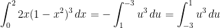
The problem with this set-up, of course, is that the letter $x$ has already been reserved as the right endpoint for this definite integral. Therefore, inside the integral, we should choose any other letter — just not $x$ — as the dummy variable.

Which sets up my one-liner: “In the words of the great philosopher Jean-Luc Picard: Plenty of letters left in the alphabet.”

We then write the integral as something like

$\displaystyle \int_0^x 3t^2 \, dt$

and then get on with the business of finding $F(x)$ .