The following problem appeared in Volume 97, Issue 3 (2024) of Mathematics Magazine.
Two points and are chosen at random (uniformly) from the interior of a unit circle. What is the probability that the circle whose diameter is segment lies entirely in the interior of the unit circle?
Let be the interior of the circle centered at the origin with radius . Also, let denote the circle with diameter , and let be the distance of from the origin.
In the previous post, we showed that
.
To find , I will integrate over this conditional probability:
,
where is the cumulative distribution function of . For ,
.
Therefore,
.
To calculate this integral, I’ll use the trigonometric substitution . Then the endpoints and become and . Also, . Therefore,
,
confirming the answer I had guessed from simulations.
The following problem appeared in Volume 97, Issue 3 (2024) of Mathematics Magazine.
Two points and are chosen at random (uniformly) from the interior of a unit circle. What is the probability that the circle whose diameter is segment lies entirely in the interior of the unit circle?
As discussed in a previous post, I guessed from simulation that the answer is . Naturally, simulation is not a proof, and so I started thinking about how to prove this.
My first thought was to make the problem simpler by letting only one point be chosen at random instead of two. Suppose that the point is fixed at a distance from the origin. What is the probability that the point , chosen at random, uniformly, from the interior of the unit circle, has the desired property?
My second thought is that, by radial symmetry, I could rotate the figure so that the point is located at . In this way, the probability in question is ultimately going to be a function of .
There is a very nice way to compute such probabilities since is chosen at uniformly from the unit circle. Let be the set of all points within the unit circle that have the desired property. Since the area of the unit circle is , the probability of desired property happening is
.
Based on the simulations discussed in the previous post, my guess was that was the interior of an ellipse centered at the origin with a semimajor axis of length and a semiminor axis of length . Now I had to think about how to prove this.
As noted earlier in this series, the circle with diameter will lie within the unit circle exactly when , where is the midpoint of . So suppose that has coordinates , where is known, and let the coordinates of be . Then the coordinates of will be
,
so that
and
.
Therefore, the condition (again, equivalent to the condition that the circle with diameter lies within the unit circle) becomes
,
which simplifies to
.
When I saw this, light finally dawned. Given two points and , called the foci, an ellipse is defined to be the set of all points so that , where is a constant. If the coordinates of , , and are , , and , then this becomes
.
Therefore, the set is the interior of an ellipse centered at the origin with and . Furthermore, is the semimajor axis of the ellipse, while the semiminor axis is equal to .
At last, I could now return to the original question. Suppose that the point is fixed at a distance from the origin. What is the probability that the point , chosen at random, uniformly, from the interior of the unit circle, has the property that the circle with diameter lies within the unit circle? Since is a subset of the interior of the unit circle, we see that this probability is equal to
.
In the next post, I’ll use this intermediate step to solve the original question.
The following problem appeared in Volume 97, Issue 3 (2024) of Mathematics Magazine.
Two points and are chosen at random (uniformly) from the interior of a unit circle. What is the probability that the circle whose diameter is segment lies entirely in the interior of the unit circle?
As discussed in the previous post, I guessed from simulation that the answer is . Naturally, simulation is not a proof, and so I started thinking about how to prove this.
My first thought was to make the problem simpler by letting only one point be chosen at random instead of two. Suppose that the point is fixed at a distance from the origin. What is the probability that the point , chosen at random, uniformly, from the interior of the unit circle, has the desired property?
My second thought is that, by radial symmetry, I could rotate the figure so that the point is located at . In this way, the probability in question is ultimately going to be a function of .
There is a very nice way to compute such probabilities since is chosen at uniformly from the unit circle. Let be the probability that the point has the desired property. Since the area of the unit circle is , the probability of desired property happening is
.
So, if I could figure out the shape of , I could compute this conditional probability given the location of the point .
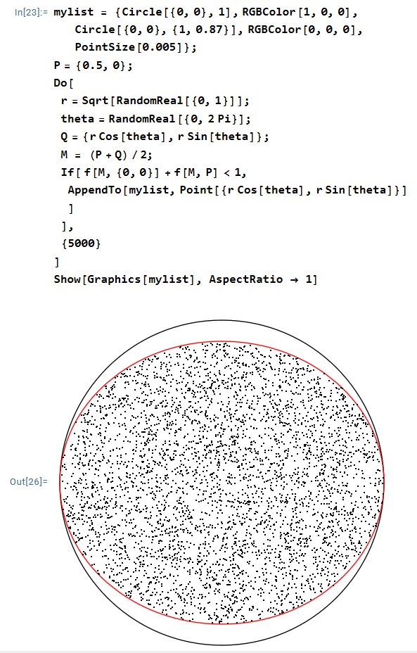
But, once again, I initially had no idea of what this shape would look like. So, once again, I turned to simulation with Mathematica. As noted earlier in this series, the circle with diameter will lie within the unit circle exactly when , where is the midpoint of . For my initial simulation, I chose to have coordinates .
To my surprise, I immediately recognized that the points had the shape of an ellipse centered at the origin. Indeed, with a little playing around, it looked like this ellipse had a semimajor axis of and a semiminor axis of about .
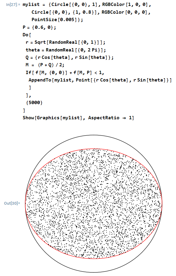
My next thought was to attempt to find the relationship between the length of the semiminor axis at the distance of from the origin. I thought I’d draw of few of these simulations for different values of and then try to see if there was some natural function connecting to my guesses. My next attempt was ; as it turned out, it looked like the semiminor axis now had a length of .
At this point, something clicked: is a Pythagorean triple, meaning that
Also, is very close to , a very familiar number from trigonometry:
So I had a guess: the semiminor axis has length . A few more simulations with different values of confirmed this guess. For instance, here’s the picture with .
Now that I was psychologically certain of the answer for , all that remain was proving that this guess actually worked. That’ll be the subject of the next post.
The following problem appeared in Volume 97, Issue 3 (2024) of Mathematics Magazine.
Two points and are chosen at random (uniformly) from the interior of a unit circle. What is the probability that the circle whose diameter is segment lies entirely in the interior of the unit circle?
As discussed in the previous post, I guessed from simulation that the answer is . Naturally, simulation is not a proof, and so I started thinking about how to prove this.
My first thought was to make the problem simpler by letting only one point be chosen at random instead of two. Suppose that the point is fixed at a distance from the origin. What is the probability that the point , chosen at random, uniformly, from the interior of the unit circle, has the desired property?
My second thought is that, by radial symmetry, I could rotate the figure so that the point is located at . In this way, the probability in question is ultimately going to be a function of .
There is a very nice way to compute such probabilities since is chosen at uniformly from the unit circle. Let be the probability that the point has the desired property. Since the area of the unit circle is , the probability of desired property happening is
.
So, if I could figure out the shape of , I could compute this conditional probability given the location of the point .
But, once again, I initially had no idea of what this shape would look like. So, once again, I turned to simulation with Mathematica.
First, a technical detail that I ignored in the previous post. To generate points at random inside the unit circle, one might think to let and , where the distance from the origin is chosen at random between 0 and 1 and the angle is chosen at random from . Unfortunately, this simple simulation generates too many points that are close to the origin and not enough that are close to the circle:
To see why this happened, let denote the distance of a randomly chosen point from the origin. Then the event is the same as saying that the point lies inside the circle centered at the origin with radius , so that the probability of this event should be
.
However, in the above simulation, was chosen uniformly from , so that . All this to say, the above simulation did not produce points uniformly chosen from the unit circle.
To remedy this, we employ the standard technique of using the inverse of the above function , which is clearly . In other words, we will chose randomly chosen radius to have the form , where is chosen uniformly on . In this way,
,
as required. Making this modification (highlighted in yellow) produces points that are more evenly distributed in the unit circle; any bunching of points or empty spaces are simply due to the luck of the draw.
In the next post, I’ll turn to the simulation of .
The following problem appeared in Volume 97, Issue 3 (2024) of Mathematics Magazine.
Two points and are chosen at random (uniformly) from the interior of a unit circle. What is the probability that the circle whose diameter is segment lies entirely in the interior of the unit circle?
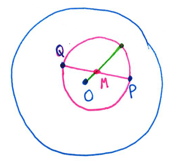
It took me a while to wrap my head around the statement of the problem. In the figure, the points and are chosen from inside the unit circle (blue). Then the circle (pink) with diameter has center , the midpoint of . Also, the radius of the pink circle is .
The pink circle will lie entirely the blue circle exactly when the green line containing the origin , the point , and a radius of the pink circle lies within the blue circle. Said another way, the condition is that the distance plus the radius of the pink circle is less than 1, or
.
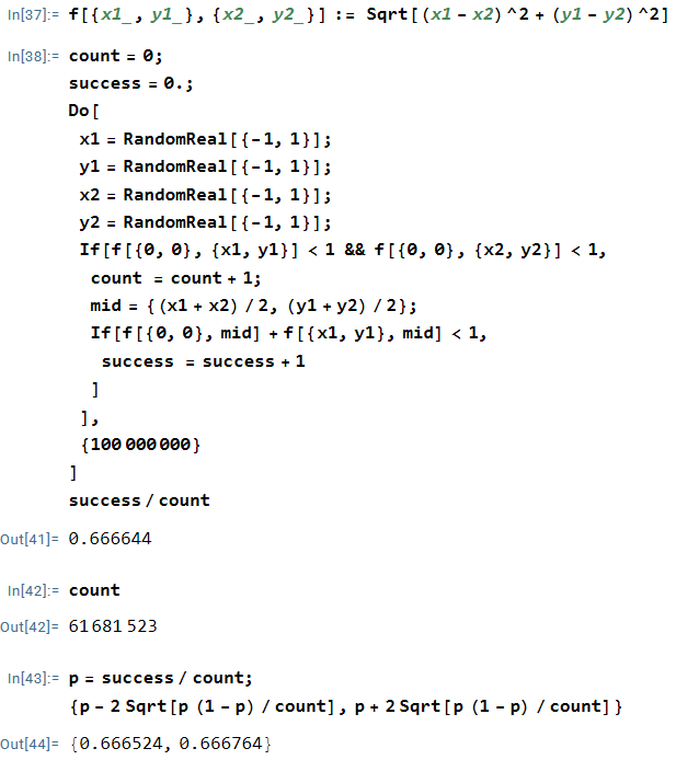
As a first step toward wrapping my head around this problem, I programmed a simple simulation in Mathematica to count the number of times that when points and were chosen at random from the unit circle.
In the above simulation, out of about 61,000,000 attempts, 66.6644% of the attempts were successful. This leads to the natural guess that the true probability is . Indeed, the 95% confidence confidence interval contains , so that the difference of from can be plausibly attributed to chance.
I end with a quick programming note. This certainly isn’t the ideal way to perform the simulation. First, for a fast simulation, I should have programmed in C++ or Python instead of Mathematica. Second, the coordinates of and are chosen from the unit square, so it’s quite possible for or or both to lie outside the unit circle. Indeed, the chance that both and lie in the unit disk in this simulation is , meaning that about of the simulations were simply wasted. So the only sense that this was a quick simulation was that I could type it quickly in Mathematica and then let the computer churn out a result. (I’ll talk about a better way to perform the simulation in the next post.)
The following problem appeared in Volume 96, Issue 3 (2023) of Mathematics Magazine.
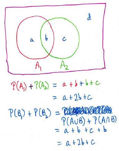
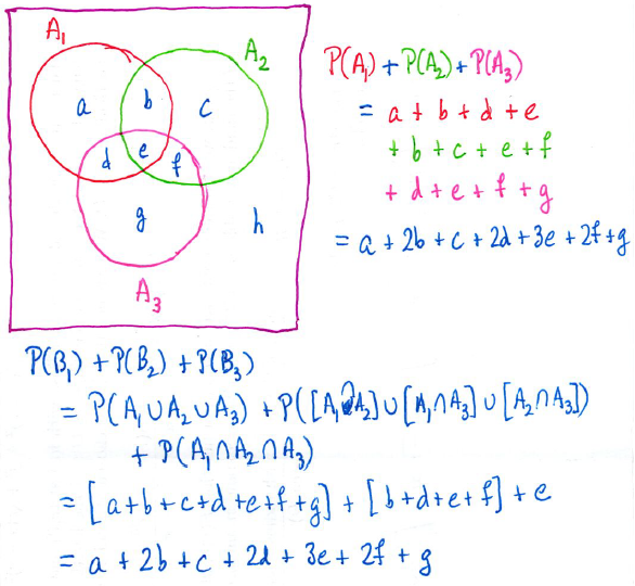
Let be arbitrary events in a probability field. Denote by the event that at least of occur. Prove that .
I’ll admit when I first read this problem, I didn’t believe it. I had to draw a couple of Venn diagrams to convince myself that it actually worked:
Of course, pictures are not proofs, so I started giving the problem more thought.
I wish I could say where I got the inspiration from, but I got the idea to define a new random variable to be the number of events from that occur. With this definition, becomes the event that , so that
At this point, my Spidey Sense went off: that’s the tail-sum formula for expectation! Since is a non-negative integer-valued random variable, the mean of can be computed by
.
Said another way, .
Therefore, to solve the problem, it remains to show that is also equal to . To do this, I employed the standard technique from the bag of tricks of writing as the sum of indicator random variables. Define
Then , so that
.
Equating the two expressions for , we conclude that , as claimed.
The following problem appeared in Volume 53, Issue 4 (2022) of The College Mathematics Journal. This was the second-half of a two-part problem.
Suppose that and are independent, uniform random variables over . Define , , , and as follows:
is uniform over ,
is uniform over ,
with and , and
.
Prove that is uniform over .
Once again, one way of showing that is uniform on is showing that if .
My first thought was that the value of depends on the value of , and so it makes sense to write as an integral of conditional probabilities:
,
where is the probability density function of . In this case, since has a uniform distribution over , we see that for . Therefore,
.
My second thought was that really has a two-part definition:
So it made sense to divide the conditional probability into these two cases:
My third thought was that these probabilities can be rewritten using the Multiplication Rule. This ordinarily has the form . For an initial conditional probability, it has the form . Therefore,
.
The definition of provides the immediate computation of and :
Also, the two-part definition of provides the next step:
We split each of these integrals into an integral from to and then an integral from to . First,
.
We now use the following: if and is uniform over , then
We observe that in the first integral, while in the second integral. Therefore,
.
For the second integral involving , we again split into two subintegrals and use the fact that if is uniform on , then
Therefore,
.
Combining, we conclude that
,
from which we conclude that is uniformly distributed on .
As I recall, this took a couple days of staring and false starts before I was finally able to get the solution.
The following problem appeared in Volume 53, Issue 4 (2022) of The College Mathematics Journal. This was the first problem that was I able to solve in over 30 years of subscribing to MAA journals.
Suppose that and are independent, uniform random variables over . Now define the random variable by
.
Prove that is uniform over . Here, is the indicator function that is equal to 1 if is true and 0 otherwise.
The first thing that went through my mind was something like, “This looks odd. But it’s a probability problem using concepts from a senior-level but undergraduate probability course. This was once my field of specialization. I had better be able to get this.”
My second thought was that one way of proving that is uniform on is showing that if .
My third thought was that really had a two-part definition:
So I got started by dividing this probability into the two cases:
.
In the last step, since , the events and are redundant: if , then will automatically be less than . Therefore, it’s safe to remove from the last probability.
Ordinarily, such probabilities are computed by double integrals over the joint probability density function of and , which usually isn’t easy. However, in this case, since and are independent and uniform over , the ordered pair is uniform on the unit square . Therefore, probabilities can be found by simply computing areas.
In this case, since the area of the unit square is 1, is equal to the sum of the areas of
,
which is depicted in green below, and
,
which is depicted in purple.
First, the area in green is a trapezoid. The intercept of the line is , and the two lengths of and on the upper left of the square are found from this intercept. The area of the green trapezoid is easiest found by subtracting the areas of two isosceles right triangles:
Second, the area in purple is an isosceles right triangle. The intercept of the line is , so that the distance from the intercept to the origin is . From this, the two lengths of and are found. Therefore, the area of the purple right triangle is .
Adding, we conclude that
.
Therefore, is uniform over .
A closing note: after going 0-for-4000 in my previous 30+ years of attempting problems submitted to MAA journals, I was unbelievably excited to finally get one. As I recall, it took me less than an hour to get the above solution, although writing up the solution cleanly took longer.
However, the above was only Part 1 of a two-part problem, so I knew I just had to get the second part before submitting. That’ll be the subject of the next post.
I end this series about numerical integration by returning to the most common (if hidden) application of numerical integration in the secondary mathematics curriculum: finding the area under the normal curve. This is a critically important tool for problems in both probability and statistics; however, the antiderivative of cannot be expressed using finitely many elementary functions. Therefore, we must resort to numerical methods instead.
In days of old, of course, students relied on tables in the back of the textbook to find areas under the bell curve, and I suppose that such tables are still being printed. For students with access to modern scientific calculators, of course, there’s no need for tables because this is a built-in function on many calculators. For the line of TI calculators, the command is normalcdf.
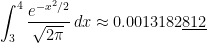
Unfortunately, it’s a sad (but not well-known) fact of life that the TI-83 and TI-84 calculators are not terribly accurate at computing these areas. For example:
TI-84:
Correct answer, with Mathematica:
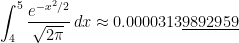
TI-84:
Correct answer, with Mathematica:
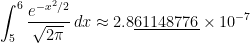
TI-84:
Correct answer, with Mathematica:
TI-84:
Correct answer, with Mathematica:
TI-84:
Correct answer, with Mathematica:
TI-84:
Correct answer, with Mathematica:
I don’t presume to know the proprietary algorithm used to implement normalcdf on TI-83 and TI-84 calculators. My honest if brutal assessment is that it’s probably not worth knowing: in the best case (when the endpoints are close to 0), the calculator provides an answer that is accurate to only 7 significant digits while presenting the illusion of a higher degree of accuracy. I can say that Simpson’s Rule with only subintervals provides a better approximation to than the normalcdf function.
For what it’s worth, I also looked at the accuracy of the NORMSDIST function in Microsoft Excel. This is much better, almost always producing answers that are accurate to 11 or 12 significant digits, which is all that can be realistically expected in floating-point double-precision arithmetic (in which numbers are usually stored accurate to 13 significant digits prior to any computations).
In my capstone class for future secondary math teachers, I ask my students to come up with ideas for engaging their students with different topics in the secondary mathematics curriculum. In other words, the point of the assignment was not to devise a full-blown lesson plan on this topic. Instead, I asked my students to think about three different ways of getting their students interested in the topic in the first place.
I plan to share some of the best of these ideas on this blog (after asking my students’ permission, of course).
This student submission again comes from my former student Angelica Albarracin. Her topic, from Pre-Algebra: probability and odds.
How can this topic be used in your students’ future courses in mathematics or science?
Probability is a topic that commonly appears in biology in the study of sexual reproduction. Both in freshman and college level biology, students are required to learn how to create and use Punnett squares. Punnett Squares are used to determine the likelihood certain alleles will appear in the offspring of 2 organisms. These alleles can do anything from determining eye color, to determining whether or not an organism will have a hereditary disease such as hemophilia.
Though statistics is not a required mathematics class for high schoolers in the state of Texas, many students will end up encountering this class in high school and/or college as it pertains directly to many fields of study such as math, biology, chemistry, and physics. One of the most important concepts in statistics is the idea of statistical significance. Using the scientific method and other techniques for conducting a survey or experiment, it is easy to analyze, and record data. However, a major component of statistics is being able to interpret the implications of any given data. One of the biggest indicators that an experiment or survey that was conducted holds real implications is its statistical significance, which is essentially a measure of the probability of observing results as extreme as what was observed.
How has this topic appeared in pop culture (movies, TV, current music, video games, etc.)?
Speed running is a category of gaming that has become hugely popular over the years in which highly skilled and knowledgeable players compete amongst each other to complete a game as fast as possible. One of the most popular of these games in this scene is Minecraft and due to Minecraft’s popularity, speed runners of this game often come within seconds of world records, meaning every small optimization could be the difference between 1st and 2nd place on the leaderboards.
Minecraft is a highly open and adventurous game primarily because each “world” is randomly generated, meaning that no two playthroughs are alike. This randomness not only encompasses world generation, but also factors into the availability of resources in the form of animals, enemies, and even ores used for building and crafting items. The most notorious section of the game where random generation plays a huge role in the speed run is in the collection of an essential item known as the ender pearl. In order to reach the final stage of the game, a minimum of 12 ender pearls are required, which can only be obtained from Endermen, a type of enemy in the game. Though ender pearls are considered an essential item for the completion of the game, it is theoretically possible to complete the game in its entirety without ever obtaining a single pearl. This is due to a unique mechanic the game uses to allow the player into its final stages.
Ender pearls are used in combination with a material called Blaze Powder to make a new item known as an Eye of Ender. Eyes of Ender are used to both locate a special portal to allow players into the “End” and to activate said portal. This portal (known as the End Portal) can only be activated with 12 eyes, but this is where the game’s inherent randomness plays an important factor. For each of the 12 slots in the portal dedicated to the placement of the eyes, there is a 10% chance that there will already be one inside, meaning the player would not need to provide one of their own. It is also important to note that while Eyes of Ender are used to locate this portal, it is completely possible to find this portal on your own, it is simply faster to use the Eye of Ender as a guide (and being faster is in the interest of speed runners). With this being said, the probability a player can complete the game without the usage of a single ender pearl is about 1 in 1 trillion!
So, what’s the big deal? Speed runners can simply obtain the required pearls and ignore this possibility, right? Normally this would be the easy answer, but it becomes a bit more complex when we consider the nature of ender pearls. As mentioned earlier, ender pearls can only be obtained from endermen, and while their exact spawn rates are unknown, they are considered to be uncommon. In addition, each endermen has only a 50% chance of dropping an ender pearl upon defeat. If you consider this with the fact that enemies primarily spawn during the night cycle of the game, it is easy to see how obtaining these pearls can take a lot of time, something a speed runner wants to avoid at all costs. Consequently, runners are often put into a scenario in which they must balance their risk and reward. Though the probability a runner will encounter an End portal with all 12 eyes built in is near impossible, the likelihood that 2 or even 3 eyes would be there is not so low. Should a speed runner devote more time to finding ender pearls, though some of their effort maybe be for nothing, or should a runner find most of the pearls, and hope the rest are at the portal waiting? In a category of gaming where every second counts, probability can be used to figure out the most optimal answer to this question, and lead hopefuls to new world records.
How can technology (YouTube, Khan Academy [khanacademy.org], Vi Hart, Geometers Sketchpad, graphing calculators, etc.) be used to effectively engage students with this topic?
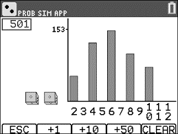
An important concept in probability is the Law of Large Numbers which states that “the relative frequency of an outcome approaches the actual probability of that outcome, as the number of repetitions gets larger” (see link below). This law can be easily observed through repeatedly tossing a coin or rolling a die, however, as the law suggests, this must be done a large amount of times. Tossing a coin 500 times in the classroom, while helpful to demonstrate this law in action, is time consuming and tedious. As a remedy to this, Texas Instruments developed an app for TI-84 graphing calculators called Probability Simulation.
In this free app, students can choose from a variety of actions to simulate such as tossing coins, rolling dice, picking marbles, and drawing cards. In the image above, the calculator is simulating the results of rolling two die. There are many useful features and settings within this app but two of the best ones are the ability to perform an action 50 at a time (indicated by +50) and a graph to keep track of the results of all previous actions. Having the ability to perform each action quickly and in large quantity makes this a much less time consuming and material intensive activity. In addition, having a graph documenting each result from previous actions also helps tremendously in demonstrating the Law of Large Numbers as it acts as a visual aid. In the picture above, the rough formation of a bell curve can be seen after 501 rolls.
References:
https://education.ti.com/en/building-concepts/activities/statistics/sequence1/law-of-large-numbershttps://www.minecraftseeds.co/stronghold-with-end-portal/https://www.speedrun.com/mc/full_game#Any_Glitchless
and
are chosen at random (uniformly) from the interior of a unit circle. What is the probability that the circle whose diameter is segment
lies entirely in the interior of the unit circle?


![= \displaystyle \frac{2}{3} \left[ u^{3/2} \right]_0^1](https://s0.wp.com/latex.php?latex=%3D+%5Cdisplaystyle+%5Cfrac%7B2%7D%7B3%7D+%5Cleft%5B++u%5E%7B3%2F2%7D+%5Cright%5D_0%5E1&bg=ffffff&fg=000000&s=0&c=20201002)
![=\displaystyle \frac{2}{3}\left[ (1)^{3/2} - (0)^{3/2} \right]](https://s0.wp.com/latex.php?latex=%3D%5Cdisplaystyle++%5Cfrac%7B2%7D%7B3%7D%5Cleft%5B+%281%29%5E%7B3%2F2%7D+-+%280%29%5E%7B3%2F2%7D+%5Cright%5D&bg=ffffff&fg=000000&s=0&c=20201002)

 . Naturally, simulation is not a proof, and so I started thinking about how to prove this.
 from the origin. What is the probability that the point
  . In this way, the probability in question is ultimately going to be a function of
  be the set of all points
  , the probability of desired property happening is
 .
. and a semiminor axis of length
  . Now I had to think about how to prove this.
 , where
  is the midpoint of
  . Then the coordinates of
  ,
,
 .
. ,
,![\displaystyle \sqrt{ \frac{1}{4} \left[ (x+t)^2 + y^2 \right]} + \sqrt{ \frac{1}{4} \left[ (x-t)^2 + y^2 \right]} < 1](https://s0.wp.com/latex.php?latex=%5Cdisplaystyle+%5Csqrt%7B+%5Cfrac%7B1%7D%7B4%7D+%5Cleft%5B+%28x%2Bt%29%5E2+%2B+y%5E2+%5Cright%5D%7D+%2B+%5Csqrt%7B+%5Cfrac%7B1%7D%7B4%7D+%5Cleft%5B+%28x-t%29%5E2+%2B+y%5E2+%5Cright%5D%7D+%3C+1&bg=ffffff&fg=000000&s=0&c=20201002)

 .
. and
and  , called the foci, an ellipse is defined to be the set of all points
  , where
  is a constant. If the coordinates of
  , and
, and  , then this becomes
 .
. and
and  . Furthermore,
  .
. .
. .
.
 .
.
 ; as it turned out, it looked like the semiminor axis now had a length of
  .
.
 is a Pythagorean triple, meaning that


 , a very familiar number from trigonometry:
 .
.
 and
and  , where the distance from the origin
  is chosen at random from
  . Unfortunately, this simple simulation generates too many points that are close to the origin and not enough that are close to the circle:
 is the same as saying that the point lies inside the circle centered at the origin with radius
  .
.![[0,1]](https://s0.wp.com/latex.php?latex=%5B0%2C1%5D&bg=ffffff&fg=000000&s=0&c=20201002) , so that
, so that  . All this to say, the above simulation did not produce points uniformly chosen from the unit circle.
 . In other words, we will chose randomly chosen radius to have the form
  , where
  is chosen uniformly on
  ,
, 
 .
.  plus the radius of the pink circle is less than 1, or
  .
.
 contains
  from
from  , meaning that about
  of the simulations were simply wasted. So the only sense that this was a quick simulation was that I could type it quickly in Mathematica and then let the computer churn out a result. (I’ll talk about a better way to perform the simulation in the next post.)
 be arbitrary events in a probability field. Denote by
  the event that at least
  of
of  occur. Prove that
  .
.
 to be the number of events from
  , so that
 .
. .
. is also equal to
  . To do this, I employed the standard technique from the
 , so that
![E(N) = \displaystyle \sum_{k=1}^n E(I_k) =\sum_{k=1}^n [1 \cdot P(A_k) + 0 \cdot P(A_k^c)] =\sum_{k=1}^n P(A_k)](https://s0.wp.com/latex.php?latex=E%28N%29+%3D+%5Cdisplaystyle+%5Csum_%7Bk%3D1%7D%5En+E%28I_k%29+%3D%5Csum_%7Bk%3D1%7D%5En+%5B1+%5Ccdot+P%28A_k%29+%2B+0+%5Ccdot+P%28A_k%5Ec%29%5D+%3D%5Csum_%7Bk%3D1%7D%5En+P%28A_k%29&bg=ffffff&fg=000000&s=0&c=20201002) .
. , as claimed.
 and
and  are independent, uniform random variables over
  ,
,  ,
,  , and
, and  as follows:
 ![[0,X]](https://s0.wp.com/latex.php?latex=%5B0%2CX%5D&bg=ffffff&fg=000000&s=0&c=20201002) ,
, ![[X,1]](https://s0.wp.com/latex.php?latex=%5BX%2C1%5D&bg=ffffff&fg=000000&s=0&c=20201002) ,
,  with
with  and
and  , and
, and .
.  if
if  .
. as an integral of conditional probabilities:
 ,
, is the probability density function of
  for
for  . Therefore,
 .
.


 . For an initial conditional probability, it has the form
  . Therefore,
 .
. and
and  :
:


 to
to 
 .
.![[0,x]](https://s0.wp.com/latex.php?latex=%5B0%2Cx%5D&bg=ffffff&fg=000000&s=0&c=20201002) , then
, then
 in the first integral, while
  in the second integral. Therefore,
 .
. is uniform on
 ![[x,1]](https://s0.wp.com/latex.php?latex=%5Bx%2C1%5D&bg=ffffff&fg=000000&s=0&c=20201002) , then
, then


 .
.
![= \displaystyle \int_0^t [x + (t-x)] \, dx + \int_t^1 t \, dx](https://s0.wp.com/latex.php?latex=%3D++%5Cdisplaystyle+%5Cint_0%5Et+%5Bx+%2B+%28t-x%29%5D++%5C%2C+dx+%2B+%5Cint_t%5E1+t+%5C%2C+dx&bg=ffffff&fg=000000&s=0&c=20201002)


 ,
, by
by .
.![{\bf 1}[S]](https://s0.wp.com/latex.php?latex=%7B%5Cbf+1%7D%5BS%5D&bg=ffffff&fg=000000&s=0&c=20201002) is the indicator function that is equal to 1 if
is the indicator function that is equal to 1 if  is true and 0 otherwise.
 if
if 


 .
. and
and  are
are  is uniform on the unit square
 ![[0,1] \times [0,1]](https://s0.wp.com/latex.php?latex=%5B0%2C1%5D+%5Ctimes+%5B0%2C1%5D&bg=ffffff&fg=000000&s=0&c=20201002) . Therefore, probabilities can be found by simply computing areas.
. Therefore, probabilities can be found by simply computing areas. is equal to the sum of the areas of
 ![\{(x,y) \in [0,1] \times [0,1] : x \le y \le x + t \}](https://s0.wp.com/latex.php?latex=%5C%7B%28x%2Cy%29+%5Cin+%5B0%2C1%5D+%5Ctimes+%5B0%2C1%5D+%3A+x+%5Cle+y+%5Cle+x+%2B+t+%5C%7D&bg=ffffff&fg=000000&s=0&c=20201002) ,
,![\{(x,y) \in [0,1] \times [0,1] : y \le x + t - 1 \}](https://s0.wp.com/latex.php?latex=%5C%7B%28x%2Cy%29+%5Cin+%5B0%2C1%5D+%5Ctimes+%5B0%2C1%5D+%3A+y+%5Cle+x+%2B+t+-+1+%5C%7D&bg=ffffff&fg=000000&s=0&c=20201002) ,
,
 intercept of the line
  is
is  , and the two lengths of
  on the upper left of the square are found from this
  is
is  , so that the distance from the
  .
. .
. cannot be expressed using finitely many elementary functions. Therefore, we must resort to numerical methods instead.


 subintervals provides a better approximation to
  than the normalcdf function.