Engaging students: Parabolas

In my capstone class for future secondary math teachers, I ask my students to come up with ideas for engaging their students with different topics in the secondary mathematics curriculum. In other words, the point of the assignment was not to devise a full-blown lesson plan on this topic. Instead, I asked my students to think about three different ways of getting their students interested in the topic in the first place.

I plan to share some of the best of these ideas on this blog (after asking my students’ permission, of course).

This student submission comes from my former student Claire McMahon. Her topic, from Precalculus: parabolas.

The parabola took a long time to get to us and took a few thinkers to really get the idea down. This website that I found really nailed the dates and also simplified the rational that led up to the parabola as we know it today. The history of the parabola is as follows:

The parabola was explored by Menaechmus (380 BC to 320 BC), who was a pupil of Plato and Eudoxus. He was trying to duplicate the cube by finding the side of the cube that has an area double the cube. Instead, Menaechmus solved it by finding the intersection of the two parabolas x²=y and y²=2x. Euclid (325 BC to 265 BC) wrote about the parabola. Apollonius (262 BC to 190 BC) named the parabola. Pappus (290 to 350) considered the focus and directrix of the parabola. Pascal (1623 to 1662) considered the parabola as a projection of a circle. Galileo (1564 to 1642) showed that projectiles falling under uniform gravity follow parabolic paths. Gregory (1638 to 1675) and Newton (1643 to 1727) considered the properties of a parabola.

This really got me to thinking what it really took to figure out the derivation of the formula and even for the graph of the parabola. I find it interesting that the idea had to travel through seven genius minds to come to all of the properties that the parabola holds to this day.

This same website led me to another use of the parabola, other than to describe a projectile’s path. The use of suspension bridges relies heavily on a parabolic model. Other parabolic models would include the satellite dishes and even all types of lights. Have you ever thought that every single place that light bulb reflects is a reflection off a point from the focus to the parabola to create your beam of light!! Pretty cool!! So you might ask why do I need to know anything about parabolas? There is your answer; it’s used in everyday life. Here are a couple of examples from the website that I found interesting:

One of the “real world” applications of parabolas involves the concept of a 3D parabolic reflector in which a parabola is revolved about its axis (the line segment joining the vertex and focus). The shape of car headlights, mirrors in reflecting telescopes, and television and radio antennae (such as the one below) all utilize this property.

Antenna of a Radio Telescope

All incoming rays parallel to the axis of the parabola are reflected through the focus.

Flashlights & Headlights

In terms of a car headlight, this property is used to reflect the light rays emanating from the focus of the parabola (where the actual light bulb is located) in parallel rays.

Here are the specs on the suspension bridge:

Hold up a chain by both ends and you’ll get a curve. What kind of curve is it? You might say it is a parabola – Galileo Galili believed it was a parabola. Yet, Galileo was wrong!!!! That curve is NOT a parabola. It is a catenary.It makes sense that you would think that the curved chain is a parabola. Both the catenary and the parabola have similar properties. Both curves have a single low point. They both have a vertical line of symmetry, they at least appear to be continuous and differentiable throughout, and the slope is steeper as we move away from the low point, but it never becomes vertical.So, how is the curve of the cable in a suspension bridge a parabola? When the structure is being built and the main cables are attached to the towers, the curve is a catenary. But when the cables are attached to the deck with hangers, it is no longer a catenary. The curve of the cables become the curve of a parabola. Unlike the catenary, which is curving under its own weight, the parabola is curving not just under its own weight, but also curving from holding up the weight of the deck. The cable of a suspension bridge is under tension from holding up the bridge.Therefore, the cables of a suspension bridge is a parabola, because the weight of the deck is equally distributed on the curve.

I never really knew that there was a difference between the two and now I know that there are certain properties that made it down through the ages that hold true today. This was a very enlightening subject matter.

Website used: http://www.carondelet.pvt.k12.ca.us/Family/Math/03210/page2.htm

A curious square root (Part 2)

There are two natural ways of computing $\sin 15^o$ using trig identities.

Method #1.

$\sin 15^o = \sin(45^o - 30^o)$

$\sin 15^o = \sin 45^o \cos 30^o - \cos 45^o \sin 30^o$

$\sin 15^o = \displaystyle \frac{\sqrt{2}}{2} \cdot \frac{1}{2} - \frac{\sqrt{2}}{2} \cdot \frac{1}{2}$

$\sin 15^o = \displaystyle \frac{\sqrt{6} - \sqrt{2}}{4}$

The same expression would be obtained if we had started with $15^o = 60^o - 45^o$ .

Method #2. Since $15^o$ is in the first quadrant,

$\sin 15^o = \sin \displaystyle \left( \frac{1}{2} \cdot 30^o \right)$

$\sin 15^o = \displaystyle \sqrt{ \frac{1 - \cos 30^o}{2} }$

$\sin 15^o = \displaystyle \sqrt{ \frac{1 - \displaystyle \frac{\sqrt{3}}{2}}{2} }$

$\sin 15^o = \displaystyle \sqrt{ \frac{2 -\sqrt{3}}{4} }$

$\sin 15^o = \displaystyle \frac{ \sqrt{2 -\sqrt{3}}}{2}$

Therefore,

$\displaystyle \frac{\sqrt{6} - \sqrt{2}}{4} = \displaystyle \frac{ \sqrt{2 -\sqrt{3}}}{2}$ ,

which may be verified by squaring both sides.

Non-geometric infinite series (Part 12)

I conclude this series of posts with thoughts about infinite series which use reciprocals of positive integers. I offer this post for the enrichment of talented Precalculus students who have exhibited mastery of geometric series.

Geometric. As we’ve discussed at length, the series

$1 + \displaystyle \frac{1}{2} + \frac{1}{4} + \frac{1}{8} + \frac{1}{16} + \dots$

converges and is in fact equal to $2$ .

Harmonic. Including the reciprocals of all positive integers is called a harmonic series:

$1 + \displaystyle \frac{1}{2} + \frac{1}{3} + \frac{1}{4} + \frac{1}{5} + \dots$

As shown in the link to the MathWorld website, this series actually diverges, even though the terms get smaller and smaller.

So we’ve made an observation: if too many reciprocals are included, the series diverges. But if we take enough of them away, then we can still end up with a series that is infinite but converges.

Squares. Let’s now consider the reciprocals of perfect squares:

$1 + \displaystyle \frac{1}{4} + \frac{1}{9} + \frac{1}{16} + \frac{1}{25} + \dots$

Clearly, we’ve taken away a lot of the terms of the harmonic series? Have we taken enough away so that the series converges? It turns out that the answer is yes. And the answer is precisely what you’d think it should be (not): $\pi^2/6$ . This is just another way that the circumference of a circle has an odd way of appearing in the most unexpected of places.

The proof that this series equals $\pi^2/6$ requires the clever use of Parseval’s theorem from Fourier analysis.

Fourth Powers. Let’s now turn to the reciprocals of fourth powers:

$1 + \displaystyle \frac{1}{16} + \frac{1}{81} + \frac{1}{256} + \frac{1}{625} + \dots$

By the Direct Comparison Test and the series for reciprocals of squares, this series converges. Using Parseval’s theorem, it can be shown that the answer is $\pi^4/90$ .

Cubes. Now let’s investigate the reciprocals of cubes:

$1 + \displaystyle \frac{1}{8} + \frac{1}{27} + \frac{1}{64} + \frac{1}{125} + \dots$

Again by the Direct Comparison Test and the series for reciprocals for squares, this series must converge. This sum is called Apéry’s constant. However, and amazingly, no one knows what the answer is. Of course, a computer can be programmed to evaluate this series to as many decimal places as desired. According to Wikipedia, this sum was evaluated to over 100 billion decimal places in 2010. However, to the best of my knowledge, no one has figured out if there’s a simple way of writing the answer, like $\pi^2/6$ or $\pi^4/90$ .

So if you figure out a simple way to evaluate Apéry’s constant, feel free to call me collect.

The previous four series are example of Riemann’s zeta function, which is of central importance in number theory and is the focus of the celebrated Riemann Hypothesis, for which a solution is worth a cool $1 million.

Primes. Now let’s consider the reciprocals of primes:

$\displaystyle \frac{1}{2} + \frac{1}{3} + \frac{1}{5} + \frac{1}{7} + \frac{1}{11} + \dots$

As noted above, the harmonic series diverges, but if we remove enough terms from the harmonic series, then it’s possible to make an infinite series that converges. So the central question is, did we remove enough fractions (by taking away all of the composite denominators) so that the series converges?

Surprisingly, the answer is no: the sum of the reciprocals of the primes actually diverges. The proof actually requires a graduate-level class in analytic number theory.

By no means would I expect high school students to master all of the above facts. As noted above, the subject of this post is mostly for the enrichment of high school students who have mastered infinite geometric series.

That said, students who know the following facts from Precalculus will be well-served when they reach calculus and other university-level mathematics courses.

They should either know the formula for an infinite geometric series or else be able to quickly derive it.
They should know that not every infinite geometric series is geometric.
They should know that not every infinite series converges.
They should be familiar with the meaning of the terms converge and diverge.

Formula for an infinite geometric series (Part 11)

Many math majors don’t have immediate recall of the formula for an infinite geometric series. They often can remember that there is a formula, but they can’t recollect the details. While it’s I think it’s OK that they don’t have the formula memorized, I think is a real shame that they’re also unaware of where the formula comes from and hence are unable to rederive the formula if they’ve forgotten it.

In this post, I’d like to give some thoughts about why the formula for an infinite geometric series is important for other areas of mathematics besides Precalculus. (There may be others, but here’s what I can think of in one sitting.)

1. An infinite geometric series is actually a special case of a Taylor series. (See https://meangreenmath.com/2013/07/05/reminding-students-about-taylor-series-part-5/ for details.) Therefore, it would be wonderful if students learning Taylor series in Calculus II could be able to relate the new topic (Taylor series) to their previous knowledge (infinite geometric series) which they had already seen in Precalculus.

2. An infinite geometric series is also a special case of the binomial series $(1+x)^n$ , when $n$ does not have to be a positive integer and hence Pascal’s triangle cannot be used to find the expansion.

3. Infinite geometric series is a rare case when an infinite sum can be found exactly. In Calculus II, a whole battery of tests (e.g., the Root Test, the Ratio Test, the Limit Comparison Test) are introduced to determine whether a series converges or not. In other words, these tests only determine if an answer exists, without determining what the answer actually is.

Throughout the entire undergraduate curriculum, I’m aware of only four types of series that can actually be evaluated exactly.

An infinite geometric series with $-1 < r < 1$
The Taylor series of a real analytic function. (Of course, an infinite geometric series is a special case of a Taylor series.)
A telescoping series. For example, using partial fractions and cancelling a bunch of terms, we find that

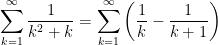
$\displaystyle \sum_{k=1}^\infty \frac{1}{k^2+k} = \displaystyle \sum_{k=1}^\infty \left( \frac{1}{k} - \frac{1}{k+1} \right)$

$\displaystyle \sum_{k=1}^\infty \frac{1}{k^2+k} = \displaystyle \left( 1 - \frac{1}{2} \right) + \left( \frac{1}{2} - \frac{1}{3} \right) \dots$

$\displaystyle \sum_{k=1}^\infty \frac{1}{k^2+k} = 1$

An infinite series that arises from Parseval’s theorem in Fourier analysis.

4. Infinite geometric series are essential for proving basic facts about decimal representations that we often take for granted.

We can justify why $0.\overline{9} = 1$ . See https://meangreenmath.com/2013/09/03/why-does-0-999-1-part-3/ for details.
Along with the Direct Comparison Test, we can be used to justify why a decimal representation $0.d_1d_2d_3\dots$ actually converges and must correspond to a real number. See https://meangreenmath.com/2013/09/01/why-does-0-999-1-part-1/ for details.
We can prove that a fraction of the form $\displaystyle \frac{M}{10^k-1}$ must have a repeating block of length $k$ which contains the digits of $M$ . See https://meangreenmath.com/2013/08/22/thoughts-on-17-and-other-rational-numbers-part-5/ for details.
Going the other direction, we can also convert an repeating decimal representation into a fraction. See https://meangreenmath.com/2013/08/21/thoughts-on-17-and-other-rational-numbers-part-4/ for details.
We can also find representations in other bases besides base 10. See https://meangreenmath.com/2013/08/17/calculator-errors-when-close-isnt-close-enough-part-2 for an example of a repeating binary representation.

5. Properties of an infinite geometric series are needed to find the mean and standard deviation of a geometric random variable, which is used to predict the number of independent trials needed before an event happens. This is used for analyzing the coupon collector’s problem, among other applications.

Formula for an infinite geometric series (Part 10)

I conclude this series of posts by considering the formula for an infinite geometric series. Somewhat surprisingly (to students), the formula for an infinite geometric series is actually easier to remember than the formula for a finite geometric series.

One way of deriving the formula parallels the derivation for a finite geometric series. If $a_1, a_2, a_3, \dots$ are the first terms of an infinite geometric sequence, let

$S = a_1 + a_2 + a_3 + \dots$

Recalling the formula for an geometric sequence, we know that

$a_2 = a_1 r$

$a_3 = a_1 r^2$

$\vdots$

Substituting, we find

$S = a_1 + a_1 r+ a_1 r^2 \dots$

Once again, we multiply both sides by $-r$ .

$-rS = -a_1r - a_1 r^2- a_1 r^3 \dots$

Next, we add the two equations. Notice that almost everything cancels on the right-hand side… except for the leading term $a_1$ . (Unlike yesterday’s post, there is no “last” term that remains since the series is infinite.) Therefore,

$S - rS = a_1$

$S(1-r) = a_1$

$S = \displaystyle \frac{a_1}{1-r}$

A quick pedagogical note: I find that this derivation “sells” best to students when I multiply by $-r$ and add, as opposed to multiplying by $r$ and subtracting.

The above derivation is helpful for remembering the formula but glosses over an extremely important detail: not every infinite geometric series converges. For example, if $a_1 = 1$ and $r = 2$ , then the infinite geometric series becomes

$1 + 2 + 4 + 8 + 16 + \dots$ ,

which clearly does not have a finite answer. We say that this series diverges. In other words, trying to evaluate this sum makes as much sense as trying to divide a number by zero: there is no answer.

That said, it can be shown that, as long as $-1 < r < 1$ , then the above geometric series converges, so that

$a_1 + a_1 r + a_1 r^2 + \dots = \displaystyle \frac{a_1}{1-r}$

The formal proof requires the use of the formula for a finite geometric series:

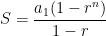
$a_1 + a_1 r + a_1 r^2 + \dots + a_1 r^{n-1} = \displaystyle \frac{a_1(1-r^n)}{1-r}$

We then take the limit as $n \to \infty$ :

$\displaystyle \lim_{n \to \infty} a_1 + a_1 r + a_1 r^2 + \dots + a_1 r^{n-1} = \displaystyle \lim_{n \to \infty} \frac{a_1(1-r^n)}{1-r}$

$a_1 + a_1 r + a_1 r^2 + \dots = \displaystyle \lim_{n \to \infty} \frac{a_1(1-r^n)}{1-r}$

On the right-hand side, the only piece that contains an $n$ is the term $r^n$ . If $-1 < r < 1$ , then $r^n \to 0$ as $n \to \infty$ . (This limit fails, however, if $r \ge 1$ or $r \le -1$ .) Therefore,

$a_1 + a_1 r + a_1 r^2 + \dots = \displaystyle \lim_{n \to \infty} \frac{a_1(1-0)}{1-r} = \displaystyle \frac{a_1}{1-r}$

Formula for an infinite geometric series (Part 9)

I continue this series of posts by considering the formula for an infinite geometric series. Somewhat surprisingly (to students), the formula for an infinite geometric series is actually easier to remember than the formula for a finite geometric series.

One way of deriving the formula parallels yesterday’s post. If $a_1, a_2, a_3, \dots$ are the first terms of an infinite geometric sequence, let

$S = a_1 + a_2 + a_3 + \dots$

Recalling the formula for an geometric sequence, we know that

$a_2 = a_1 r$

$a_3 = a_1 r^2$

$\vdots$

Substituting, we find

$S = a_1 + a_1 r+ a_1 r^2 \dots$

For example, if $a_1 = \displaystyle \frac{1}{2}$ and $r = \displaystyle \frac{1}{2}$ , we have

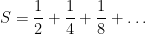
$S = \displaystyle \frac{1}{2} + \frac{1}{4} + \frac{1}{8} + \dots$

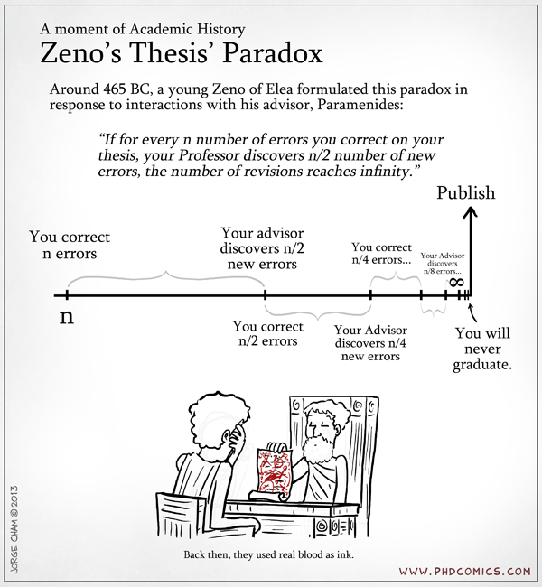
This is perhaps the world’s most famous infinite series, as this is the subject of Zeno’s paradox. When I teach infinite series in class, I often engage the students by reminding students about Zeno’s paradox and then show them this clip from the 1994 movie I.Q.

This clip is almost always a big hit with my students.

Even after showing this clip, some students resist the idea that an infinite series can have a finite answer. For such students, I use a physical demonstration: I walk half-way across the classroom, then a quarter, and so on… until I walk head-first into a walk at full walking speed. The resulting loud thud usually confirms for students that an infinite sum can indeed have a finite answer.

P.S. PhD Comics recently had a cartoon concerning Zeno’s paradox. Source: http://www.phdcomics.com/comics/archive.php?comicid=1610

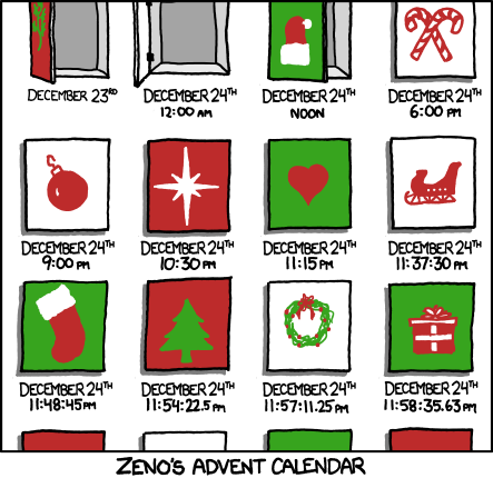
Here’s another one. Source: http://www.xkcd.com/994/

Formula for a finite geometric series (Part 8)

As I’ve said before, I’m not particularly a fan of memorizing formulas. Apparently, most college students aren’t fans either, because they often don’t have immediate recall of certain formulas from high school when they’re needed in the collegiate curriculum.

While I’m not a fan of making students memorize formulas, I am a fan of teaching students how to derive formulas. Speaking for myself, if I ever need to use a formula that I know exists but have long since forgotten, the ability to derive the formula allows me to get it again.

Which leads me to today’s post: the derivation of the formulas for the sum of a finite geometric series. This topic is commonly taught in Precalculus but, in my experience, is often forgotten by students years later when needed in later classes.

Like its counterpart for arithmetic series, the formula for a finite geometric series can be derived using the patented Bag of Tricks. Socrates gave the Bag of Tricks to Plato, Plato gave it to Aristotle, it passed down the generations, my teacher taught the Bag of Tricks to me, and I teach it to my students.

If $a_1, \dots, a_n$ are the first $n$ terms of an geometric sequence, let

$S = a_1 + a_2 + a_3 + \dots + a_{n-1} + a_n$

Recalling the formula for an geometric sequence, we know that

$a_2 = a_1 r$

$a_3 = a_1 r^2$

$\vdots$

$a_{n-1} = a_1 r^{n-2}$

$a_n = a_1 r^{n-1}$

Substituting, we find

$S = a_1 + a_1 r+ a_1 r^2 \dots + a_1 r^{n-2} + a_1 r^{n-1}$

At this point, we use something different from the patented Bag of Tricks: we multiply both sides by $-r$ .

$-rS = -a_1r - a_1 r^2- a_1 r^3 \dots - a_1 r^{n-1} - a_1 r^n$

Next, we add the two equations. Notice that almost everything cancels on the right-hand side. The $a_1 r$ cancel, the $a_1 r^2$ cancel, yada yada yada, and the $a_1 r^{n-1}$ cancel. The only terms that remain are $a_1$ and $-a_1 r^n$ . So

$S - rS = a_1 - a_1 r^n$

$S(1-r) = a_1 (1- r^n)$

$S = \displaystyle \frac{a_1 ( 1-r^n) }{1-r}$

A quick pedagogical note: I find that this derivation “sells” best to students when I multiply by $-r$ and add, as opposed to multiplying by $r$ and subtracting.

This formula is also a straightforward consequence of the factorization formula

$x^n - y^n = (x-y)(x^{n-1} + x^{n-2} y + \dots +x y^{n-2} + y^{n-1})$

Just let $x=1$ and $y=r$ , and then multiply both sides by the first term $a_1$ .

However, in my experience, most students don’t have instant recall of this formula either. They can certainly remember the formula for the difference of two squares (which is a special case of the above formula), but they often can’t remember that the difference of two cubes has a formula. (And, while I’m on the topic, they also can’t remember that the sum of two cubes can always be factored.)

Pedagogically, the most common mistake that I see students make when using this formula is using the wrong exponent on the right-hand side. For example, suppose the problem is to simplify

$48 +24+ 12 + 6 + 3 + 1.5 + 0.75 + 0.375$

Here’s the common mistake: student solve for $n$ using the formula for a geometric sequence. They solve for the unknown exponent (often using logarithms) and find that $0.375 = 48 (0.5)^7$ . They conclude that $n=7$ , and then plug into for formula for a geometric series:

$S = \displaystyle \frac{48 ( 1-(0.5)^7) }{1-0.5} = 95.25$ (incorrect)

This answer is clearly wrong, since the sum of the original series must have a $5$ in the thousandths place. The answer $95.25$ is the correct answer to the wrong question — that’s the sum of the first seven terms of the sequence (stopping at $0.75$ ), but the original series has eight terms. Using the formula correctly, we find

$S = \displaystyle \frac{48 ( 1-(0.5)^8) }{1-0.5} = 95.625$ (correct)

Not surprisingly, the difference between the incorrect and correct answers is $0.375$ , the eighth term.

To help students avoid this mistake, I re-emphasize that the number $n$ stands for the number of terms in the series. In particular, it does not mean the exponent needed to give the last term in the series. That exponent, of course, is $n-1$ , not $n$ .

Formula for an arithmetic series (Part 7)

As we’ve discussed, the formula for an arithmetic series is

$S_n = \displaystyle \frac{n}{2} (2a_1 + [n-1] d) = \displaystyle \frac{n}{2} (a_1 + a_n)$ ,

where $n$ is the number of terms, $a_1$ is the first term, $d$ is the common difference, and $a_n$ is the last term. This formula may be more formally expressed as

$S = \displaystyle \sum_{k=1}^n a_k = \displaystyle \frac{n}{2} (2a_1 + [n-1] d) = \displaystyle \frac{n}{2} (a_1 + a_n)$

For homework and on tests, students are asked to directly plug into this formula and to apply this problem with word problems, like finding the total number of seats in an auditorium with 50 rows, where there are 12 seats in the front row and each row has two more seats than the row in front of it.

In my opinion, the ability to solve questions like the one below is the acid test for determining whether a student — who I assume can solve routine word problems like the one above — really understands series or is just familiar with series. In other words, if a student can solve routine word problems but is unable to handle a problem like the one below, then there’s still room for that student’s knowledge of series to deepen.

Calculate $\displaystyle \sum_{k=11}^{60} (5k - 2)$

There are two reasonable approaches for solving this problem.

Solution #1. Notice that $5k - 2 = 5(k-1) + 5 - 2 = 3 + 5(k-1)$ . So this is really an arithmetic series whose first term is $3$ and whose common difference is $5$ . Therefore,

$S = \displaystyle \sum_{k=1}^{60} a_k = \displaystyle \frac{60}{2} (2[3] + [60-1] 5)=9030$

However, I’m supposed to start the series on $k=11$ , not $k=1$ . That means that I need to subtract off the first ten terms of the above series. Now

$S = \displaystyle \sum_{k=1}^{10} a_k = \displaystyle \frac{10}{2} (2[3] + [10-1] 5)= 255$

Finally,

$\displaystyle \sum_{k=11}^{60} a_k = \displaystyle \sum_{k=1}^{60} a_k - \displaystyle \sum_{k=1}^{10} a_k = 9030 - 255 = 8775$

Solution #2. Writing out the terms, we see that

$\displaystyle \sum_{k=11}^{60} (5k - 2) = (5[11]-2) + (5[12]-2) + \dots + (5[60]-2)$

$\displaystyle \sum_{k=11}^{60} (5k - 2) = 53+58 + \dots +298$

The right-hand side is an arithmetic series whose “first” term is $53$ and whose last ( $50$ th) term is $298$ . Therefore,

$\displaystyle \sum_{k=11}^{60} (5k - 2) = \frac{50}{2} (53+298) = 8775$

Of the two solutions, I suppose I have a mild preference for the first, as the second solution won’t work for something like $\displaystyle \sum_{k=11}^{60} k^2$ . However, both solution demonstrate that the student is actually thinking about the meaning of the series instead of just plugging numbers in a formula, and so I’d be happy with either one in a Precalculus class.

Formula for an arithmetic series (Part 6)

In the previous posts of this series, I described two methods of deriving the formula

$\displaystyle \sum_{k=1}^n k = \frac{n(n+1)}{2}$

The first method concerned reversing the terms of the sum (or, almost equivalently, taking the terms in pairs). The second method used mathematical induction.

Mathematical induction can be applied to arithmetic series as well as other series. However, the catch is that you have to know the answer before proving that the answer actually is correct. By contrast, the first method did not require us to know the answer in advance — it just fell out of the calculation — but it cannot be applied to series that are not arithmetic.

Here’s a third method using the principle of telescoping series. This method has the strengths of the previous two methods: it does not require us to know the answer in advance, and it can also be applied to some other series which are not arithmetic.

To begin, consider the sum

$\displaystyle \sum_{k=1}^n [k^2 - (k-1)^2]$

At this early point, students often object, “Where did that come from?” I’ve said it before but I’ll say it again: I tell them my usual tongue-in-cheek story that this idea comes from the patented Bag of Tricks. Socrates gave the Bag of Tricks to Plato, Plato gave it to Aristotle, it passed down the generations, my teacher taught the Bag of Tricks to me, and I teach it to my students.

In any event, I will evaluate this sum in two different ways.

Step 1. Just write out the terms of the series, starting from $k=1$ and ending with $k =n$ .

$\displaystyle \sum_{k=1}^n [k^2 - (k-1)^2] = [1^2 - 0^2] + [2^2 - 1^2] + [3^2 - 2^2] + \dots + [n^2 - (n-1)^2]$

Notice that, on the right-hand side, the $1^2$ terms cancel, the $2^2$ terms cancel, and so on. In fact, almost everything cancels. The only two terms that aren’t cancelled are the $0^2$ and $n^2$ terms. Therefore,

$\displaystyle \sum_{k=1}^n [k^2 - (k-1)^2] = n^2 - 0^2 = n^2$

Step 2. Next, we’ll rewrite the original sum by expanding out the terms inside of the sum:

$\displaystyle \sum_{k=1}^n [k^2 - (k-1)^2] = \displaystyle \sum_{k=1}^n [k^2 - (k^2 -2k + 1)]$

$\displaystyle \sum_{k=1}^n [k^2 - (k-1)^2] = \displaystyle \sum_{k=1}^n [2k-1]$

$\displaystyle \sum_{k=1}^n [k^2 - (k-1)^2] = \displaystyle \sum_{k=1}^n 2k - \displaystyle \sum_{k=1}^n 1$

$\displaystyle \sum_{k=1}^n [k^2 - (k-1)^2] = 2\displaystyle \sum_{k=1}^n k - \displaystyle \sum_{k=1}^n 1$

Step 3. Of course, these different looking answers from Steps 1 and 2 have to be the same, so let’s set them equal to each other:

$2\displaystyle \sum_{k=1}^n k - \displaystyle \sum_{k=1}^n 1 = n^2$

There is one unknown in this equation, $\displaystyle \sum_{k=1}^n k$ . The second sum is just the constant $1$ added to itself $n$ times, and so $\displaystyle \sum_{k=1}^n 1 = n$ . Therefore, we solve for the unknown:

$2 \left(\displaystyle \sum_{k=1}^n k \right) - n = n^2$

$2 \left(\displaystyle \sum_{k=1}^n k \right) = n^2 + n$

$\displaystyle \sum_{k=1}^n k = \displaystyle \frac{n^2 + n}{2}$

The beauty of this approach is that this approach can be continued. For example, to obtain $\displaystyle \sum_{k=1}^n k^2$ , we begin with

$\displaystyle \sum_{k=1}^n [k^3 - (k-1)^3]$

Step 1. By telescoping series,

$\displaystyle \sum_{k=1}^n [k^3 - (k-1)^3] = n^3 - 0^3 = n^3$

Step 2. Using the binomial theorem,

$\displaystyle \sum_{k=1}^n [k^3 - (k-1)^3] = \displaystyle \sum_{k=1}^n [k^3 - (k^3 -3k^2+3k- 1)]$

$\displaystyle \sum_{k=1}^n [k^2 - (k-1)^2] = 3\displaystyle \sum_{k=1}^n k^2 - 3\displaystyle \sum_{k=1}^n k + \displaystyle \sum_{k=1}^n 1$

$\displaystyle \sum_{k=1}^n [k^2 - (k-1)^2] = 3\displaystyle \sum_{k=1}^n k^2 - 3\left( \frac{n(n+1)}{2} \right) + n$

Step 3. Setting these two expressions equal to each other,

$3\displaystyle \sum_{k=1}^n k^2 - 3\left( \frac{n(n+1)}{2} \right) + n= n^3$

And we eventually conclude that:

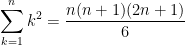
$\displaystyle \sum_{k=1}^n k^2 = \displaystyle \frac{n(n+1)(2n+1)}{6}$

And then this could be continued to obtain closed-form expressions for higher exponents of $k$ .

Formula for an arithmetic series (Part 5)

In Precalculus, Discrete Mathematics or Real Analysis, an arithmetic series is often used as a student’s first example of a proof by mathematical induction. Recall, from Wikipedia:

Mathematical induction is a method of mathematical proof typically used to establish a given statement for all natural numbers. It is done in two steps. The first step, known as the base case, is to prove the given statement for the first natural number. The second step, known as the inductive step, is to prove that the given statement for any one natural number implies the given statement for the next natural number. From these two steps, mathematical induction is the rule from which we infer that the given statement is established for all natural numbers.

The simplest and most common form of mathematical induction infers that a statement involving a natural number n holds for all values of n. The proof consists of two steps:

The basis (base case): prove that the statement holds for the first natural number $n$ . Usually, $n=0$ or $n=1$ .

The inductive step: prove that, if the statement holds for some natural number $n$ , then the statement holds for $n+1$ .

The hypothesis in the inductive step that the statement holds for some $n$ is called the induction hypothesis (or inductive hypothesis). To perform the inductive step, one assumes the induction hypothesis and then uses this assumption to prove the statement for $n+1$ .

As an inference rule, mathematical induction can be justified as follows. Having proven the base case and the inductive step, then any value can be obtained by performing the inductive step repeatedly. It may be helpful to think of the domino effect. Consider a half line of dominoes each standing on end, and extending infinitely to the right. Suppose that:

The first domino falls right.

If a (fixed but arbitrary) domino falls right, then its next neighbor also falls right.

With these assumptions one can conclude (using mathematical induction) that all of the dominoes will fall right.

Mathematical induction… works because $n$ is used to represent an arbitrary natural number. Then, using the inductive hypothesis, i.e. that $P(n)$ is true, show $P(k+1)$ is also true. This allows us to “carry” the fact that $P(0)$ is true to the fact that $P(1)$ is also true, and carry $P(1)$ to $P(2)$ , etc., thus proving $P(n)$ holds for every natural number $n$ .

When students first encounter mathematical induction (in either Precalculus, Discrete Mathematics, or Real Analysis), the theorems that students are asked to prove usually fall into four categories:

Calculating a series (examples below).
Statements concerning divisibility (for example, proving that $4$ is always a factor of $5^n-1$ ).
Finding a closed-form expression for a recursively defined sequence (for example, if $a_1 = 4$ and $a_n = 3a_{n-1}$ if $n \ge 2$ , proving that $a_n = 4 \times 3^{n-1}$ 0
Statements concerning inequality (for example, proving that $n! > 4^n$ if $n \ge 9$ 0

Here’s a common first example of mathematical induction applied to an arithmetic series. Notice that the statement of the theorem matches the form $\displaystyle \frac{n}{2}(a_1 + a_n)$ seen earlier in this series (pardon the pun) of posts.

Theorem. $1 + 2 + \dots + (n-1) + n = \displaystyle \frac{n(n+1)}{2}$

Proof. Induction on $n$ .

$n = 1$ : The left-hand is simply $1$ , while the right-hand side is $\displaystyle \frac{(1)(2)}{2}$ , which is also equal to $1$ . So the base case works.

$n$ : Assume that the statement holds true for the integer $n$ .

$n+1$ . If I replace $n$ by $n+1$ in the statement of the theorem, then the right-hand side becomes

$\displaystyle \frac{(n+1)[(n+1)+1]}{2} = \displaystyle \frac{(n+1)(n+2)}{2}$

I find it helpful to describe this to students as my target. In other words, as I manipulate the left-hand side, my ultimate goal is to end up with this target. Once I have done that, then I have completed the proof.

If I replace $n$ by $n+1$ in the statement of the theorem, then the left-hand side will now end on $n+1$ instead of $n$ :

$1 + 2 + \dots + (n-1) + n + (n+1)$

Notice that we’ve seen almost all of this before, except for the extra term $n+1$ . So we will substitute using the induction hypothesis, carrying the extra $n+1$ along for the ride.

$1 + 2 + \dots + (n-1) + n + (n+1) = \displaystyle \frac{n(n+1)}{2} + (n+1)$

Now our task is, by hook or by crook, using whatever algebraic tricks we can think of to convert this last expression into the target. Most students are completely comfortable doing this, although they typically multiply out the term $n(n+1)$ unnecessarily. Indeed, many early proofs by induction are simplified by factoring out terms whenever possible — in the example below, $(n+1)$ is factored on the last step — as opposed to multiplying them out. In my experience, proofs by induction often serve as a stringent test of students’ algebra skills as opposed to their skills in abstract reasoning.

In any event, here’s the end of the proof:

$1 + 2 + \dots + (n-1) + n + (n+1) = \displaystyle \frac{n(n+1)}{2} + (n+1)$

$1 + 2 + \dots + (n-1) + n + (n+1) = \displaystyle \frac{n(n+1) + 2(n+1)}{2}$

$1 + 2 + \dots + (n-1) + n + (n+1) = \displaystyle \frac{(n+1)(n + 2)}{2}$

Mathematical induction can be used to verify formulas for series which are not arithmetic, like

$1^2 + 2^2 + \dots + (n-1)^2 + n^2 = \displaystyle \frac{n(n+1)(2n+1)}{6}$

$1^3 + 2^3 + \dots + (n-1)^3 + n^3 = \displaystyle \frac{n^2(n+1)^2}{4}$

However, the downside of a proof by induction lies in the word verify, as it’s necessary to actually know what’s going to work before proceeding with the proof.

In the next post, I’ll describe a method of obtaining these series that does not require mathematical induction.