In this series, I’m discussing how ideas from calculus and precalculus (with a touch of differential equations) can predict the precession in Mercury’s orbit and thus confirm Einstein’s theory of general relativity. The origins of this series came from a class project that I assigned to my Differential Equations students maybe 20 years ago.
In this part of the series, we will show that if the motion of a planet around the Sun is expressed in polar coordinates , with the Sun at the origin, then under Newtonian mechanics (i.e., without general relativity) the motion of the planet follows the differential equation
,
where and is a certain constant. Deriving this governing differential equation will require some principles from physics. If you’d rather skip the physics and get to the mathematics, we’ll get to solving this differential equations in a few posts.
One principle from physics that we’ll need is the Law of Conservation of Angular Momentum. Mathematically, this is expressed by
,
where is a constant. Of course, this can be written as
;
this will be used a couple times in the derivation below.
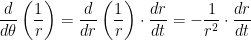
As we’ll soon see, we will need to express the second derivative in a form that depends only on . To do this, we use the Chain Rule to obtain
.
This last step used the Chain Rule in reverse:
.
To examine the second derivative , we again use the Chain Rule:
.
While far from obvious now, this will be needed when we rewrite Newton’s Second Law in polar coordinates.
In this series, I’m discussing how ideas from calculus and precalculus (with a touch of differential equations) can predict the precession in Mercury’s orbit and thus confirm Einstein’s theory of general relativity. The origins of this series came from a class project that I assigned to my Differential Equations students maybe 20 years ago.
One technique that will be necessary for this confirmation is the method of successive approximations. This will be needed in the context of a differential equation; however, we can illustrate the concept by finding the roots of a polynomial. Consider the quadratic equation
.
(Naturally, we can solve for using the quadratic formula; more on that later.) To apply the method of successive approximation, we will rewrite this so that appears on the left side and some function of appears on the right side. I will choose
, or
.
Here’s the idea of the method of successive approximations to obtain a recursively defined sequence that (hopefully) convergence to a solution of this equation:
Start with an initial guess .
Plug into the right-hand side to get a new guess, .
Plug into the right-hand side to get a new guess, .
And repeat.
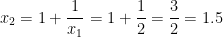
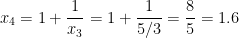
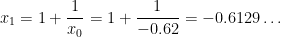
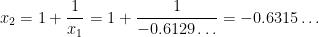
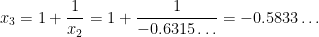
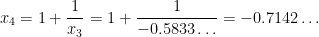
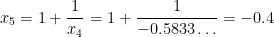
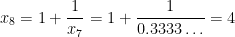
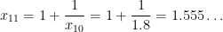
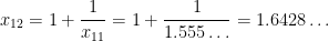
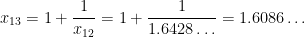
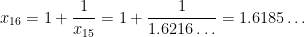
For example, suppose that we choose . Then
This sequence can be computed by entering into a calculator, then entering , and then repeatedly hitting the button.
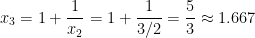
We see that the sequence appears to be converging to something, and that something is a root of the equation , which we now find via the quadratic formula:
.
So it looks like the above sequence is converging to the positive root .
(Parenthetically, you might notice that the Fibonacci sequence appears in the numerators and denominators of this sequence. As you might guess, that’s not a coincidence.)
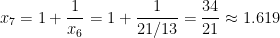
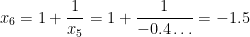
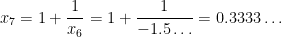
Like most numerical techniques, this method doesn’t always work like we think it would. Another solution is the negative root . Unfortunately, if we start with a guess near this root, like , the sequence unexpectedly diverges from but eventually converges to the positive root :
I should note that the method of successive approximations generally converges at a slower pace than Newton’s method. However, this method will be good enough when we use it to predict the precession in Mercury’s orbit.
A brief aside from the current series on general relativity — and the mysterious 43 seconds of arc per century in Mercury’s orbit — that turned into further discussion about angle measurement.
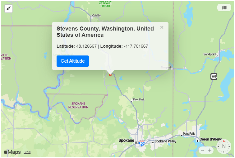
A few months ago, I received this clever postcard from someone visiting Spokane, Washington. The sender clearly knew the recipient (me) well: rather than sending me a postcard showing the jaw-dropping beauty of the Spokane area, I was impressed with the mathematical precision given for Spokane’s location.
I started wondering about exactly how precisely the postcard was measuring the location of Spokane — was it the location of City Hall or some other important landmark? — and I went to Google Maps to find out. (For what it’s worth, xkcd had a comic about this some time ago.)
And then it finally hit me, after far longer than it should have taken, that the postcard is utterly nonsensical.
We would never say that someone’s height is 4 feet, 20 inches. There are 12 inches in a foot, and so we would instead say that the height is 5 feet, 8 inches.
Likewise, when specifying an angle with minutes and seconds, there are (just like with ordinary time) 60 seconds in a minute and 60 minutes in a degree (so that there are 3600 seconds in a degree). Therefore, specifying an angle with 67′ or 66″, as in the postcard, makes absolutely no sense.
Furthermore, if converted into standard notation, we obtain a location of north, west, which is about 40 miles NNW of Spokane. (Images made by https://www.gps-coordinates.net/). Note on the conversion into decimal:
and
It’s a shame that the designer of the postcard made this error, as I genuinely thought this was a clever and aesthetically pleasing design idea for a postcard.
While I’m not sure how this mistake happened, my best guess is that the designer used the location of north, west — which is indeed in Spokane — and then misconverted from decimal notation to minutes and seconds.
In this series, I’m discussing how ideas from calculus and precalculus (with a touch of differential equations) can predict the precession in Mercury’s orbit and thus confirm Einstein’s theory of general relativity. The origins of this series came from a class project that I assigned to my Differential Equations students maybe 20 years ago.
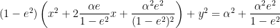
In a previous post, we showed that the polar equation
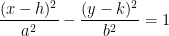
is equivalent to the rectangular equation
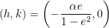
as long as . Furthermore, if , then this represents an ellipse with eccentricity whose major axis lies on the axis, with one focus located at the origin.
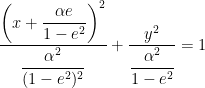
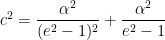
While not directly related to our discussion of precession, it turns out that this equation represents a hyperbola if . Under this assumption, and , so let me rewrite the previous equation in terms of :
This matches the form of a left-right hyperbola
,
where the center of the hyperbola is located at
Also, for a hyperbola, the distance from the center to the foci satisfies
,
so that
The two foci are located a distance to the left of the right of the center. Since it happened to happen that , this means that the origin is, once again, one of the foci of the hyperbola.
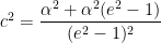
Furthermore, the eccentricity of the hyperbola is easily computed as
,
so that, once again, the well-chosen parameter is the eccentricity.
In this series, I’m discussing how ideas from calculus and precalculus (with a touch of differential equations) can predict the precession in Mercury’s orbit and thus confirm Einstein’s theory of general relativity. The origins of this series came from a class project that I assigned to my Differential Equations students maybe 20 years ago.
In the previous post, we showed that the polar equation
converts to
in rectangular coordinates. Furthermore, if , then this represents an ellipse with eccentricity whose semi-major axis lies along the axis with one focus at the origin.
It turns out that, for different non-negative values of , the same polar equation represents different conic sections. These are not particularly relevant for our study of precession, but I’m including this anyway in this series as a small tangential discussion.
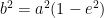
Let’s take a look at the easy case of . With this substitution, the equation in rectangular coordinates simplifies to
.
Of course, this is the equation of a circle that is centered at the origin with radius .
The other easy case is , so that . Then the equation in rectangular coordinates simplifies to
This matches the form of a parabola that opens to the left with a horizontal axis of symmetry:
.
In this case, the vertex of the parabola is located at
,
while the focus of the parabola is located a distance to the left of the vertex. In other words, the origin is the focus of the parabola. (For what it’s worth, the directrix of the parabola would be the vertical line , located to the right of the vertex.)
In this series, I’m discussing how ideas from calculus and precalculus (with a touch of differential equations) can predict the precession in Mercury’s orbit and thus confirm Einstein’s theory of general relativity. The origins of this series came from a class project that I assigned to my Differential Equations students maybe 20 years ago.
As part of our derivation, we’ll need to use the fact that, in polar coordinates, the graph of
turns out to be an ellipse if , with the origin at one focus.
We now prove this. Clearing the denominator, we obtain
.
Switching to rectangular coordinates, this becomes
Since we assumed that , we have so that
.
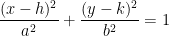
Therefore, this matches the usual form of an ellipse in rectangular coordinates
,
where the center of the ellipse is located at
,
the semi-major axis is horizontal with length
,
and the semi-minor axis is vertical with length
.
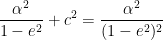
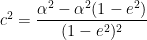
Furthermore, the distance of the foci from the center of the ellipse satisfies the equation
,
so that
From this, we derive two nice properties of the ellipse. First, looking back on previous work, we see that . Therefore, since the foci of the ellipse are distance away from the center along the major axis, we conclude that one focus of the ellipse is located at , or . That is, the origin is one focus of the ellipse. (For the little it’s worth, the other focus is located at .
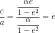
Second, the eccentricity of the ellipse is defined to be the ratio . This is now easily computed:
.
In other words, the letter was well-chosen to represent the eccentricity of the ellipse.
For what it’s worth, here’s an alternate derivation of the formulas for and . For this ellipse, the planet’s closest approach to the Sun occurs at :
,
and the planet’s further distance from the Sun occurs at :
.
Therefore, the length of the major axis of the ellipse is the sum of these two distances:
In this series, I’m discussing how ideas from calculus and precalculus (with a touch of differential equations) can predict the precession in Mercury’s orbit and thus confirm Einstein’s theory of general relativity. The origins of this series came from a class project that I assigned to my Differential Equations students maybe 20 years ago.
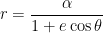
But what is precession? To explore this concept, let’s explore the graph of
for various values of , , and using Desmos. (Note that, in this context, the number does not mean Euler’s constant . The reason for choosing the letter for this parameter will become clear shortly.) Naturally, this demonstration could also be done with other tools like a graphing calculator.
I suggest beginning by setting and and altering the value of . This is the easiest behavior to explain. From the equation, is directly proportional to the distance from the origin . So, not surprisingly, increasing produces a larger graph, and decreasing produces a smaller graph.
Second, I suggest setting and but altering the value of . Starting at , the graph is a circle. This makes complete sense: if , then the equation simply becomes , so the distance from the origin is the same for all angles. However, as increases, the original circle becomes more and more stretched out. We will prove this analytically in a later post, but it turns out that, for , the graph is an ellipse, and the origin is one of the foci of the ellipse. The number is called the eccentricity of the ellipse (hence the letter ).
Again, if the value of is fixed but varies, the graph becomes either larger or smaller as becomes larger or smaller.
We notice that if and , then the denominator of
varies between and . In particular, the denominator is always positive. Therefore, the value of is least positive — the graph is closest to the origin — when the denominator is greatest. This happens when is a multiple of . So, for example, when , then is as close as the graph gets to the origin. Let’s call this closest distance ; in the context of a planet’s orbit around the sun, this represent perihelion. Then we have .
When , the graph switches from an ellipse to a parabola, where the origin is the focus of the parabola. For , the graph becomes a hyperbola. However, since we’re mostly going to be concerned with stable planetary orbits in this series, we won’t dwell too much on the case .
Third, I suggest setting , , and then alter the value of . For , the graph is simply a single ellipse. However, by changing the value of , the graph changes into a spiral.
In the above figure, the spiral stopped “spiraling” because I had asked Desmos only to show the graph between . If I had changed the upper bound to something larger than , the spiral would continue.
The precession in the spiral is defined to be the angular offset between each loop of the spiral. Clearly, this is a function of . To find this function, we again examine the function
Once again, if , then the denominator varies between and . In particular, the denominator is always positive. Therefore, the value of is least positive when the denominator is greatest, and the denominator is greatest when is a multiple of . So, for example, when , then is as close as the graph gets to the origin.
When does the graph return to its closest point to the origin next? This would occur when , or . If , then the angle of closest approach to the origin would , and the graph simply cycles over itself. However, if , then this angle will be larger than , thus producing a spiral. Indeed, the amount of precession would be equal to
.
In the picture above, . Therefore, the amount of precession would be radians . Therefore, after 19 “leafs” of the spiral, the graph would begin to cycle on top of itself.
In this series, I’m discussing how ideas from calculus and precalculus (with a touch of differential equations) can predict the precession in Mercury’s orbit and thus confirm Einstein’s theory of general relativity. The origins of this series came from a class project that I assigned to my Differential Equations students maybe 20 years ago.
This is going to be a very long series, so I’d like to provide a tree-top view of how the argument will unfold.
We begin by using three principles from Newtonian physics — the Law of Conservation of Angular Momentum, Newton’s Second Law, and Newton’s Law of Gravitation — to show that the orbit of a planet, under Newtonian physics, satisfies the initial-value problem
,
,
.
In these equations:
The orbit of the planet is in polar coordinates , where the Sun is placed at the origin.
The planet’s perihelion — closest distance from the Sun — is a distance of at angle .
The function is equal to .
is the gravitational constant of the universe.
is the mass of the Sun.
is the mass of the planet.
is the angular momentum of the planet.
The solution of this differential equation is
,
so that
.
In polar coordinates, this is the graph of an ellipse. Substituting , we see that
.
In the solution for , we have and . The number is the eccentricity of the ellipse, while is proportional to the size of the ellipse.
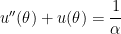
Under general relativity, the governing initial-value problem changes to
,
,
,
where is the speed of light. We will see that the solution of this new differential equation can be well approximated by
.
This last equation describes a spiral that precesses by approximately
radians per orbit
or
radians per orbit,
where is the length of the semimajor axis of the orbit.
This matches the amount of precession in Mercury’s orbit that is not explained by Newtonian physics, thus confirming Einstein’s theory of general relativity.
To the extent possible, I will take the perspective of a good student who has taken Precalculus and Calculus I. However, I will have to break this perspective a couple of times when I discuss principles from physics and derive the solutions of the above differential equations.
In this series, I’m discussing how ideas from calculus and precalculus (with a touch of differential equations) can predict the precession in Mercury’s orbit and thus confirm Einstein’s theory of general relativity. The origins of this series came from a class project that I assigned to my Differential Equations students maybe 20 years ago.
The figure below shows the (greatly exaggerated) effect of precession on a planet’s otherwise elliptical orbit. In the figure, each perihelion is precessed by an angle of . After nine orbits, the planet returns to its original position. Suppose, for the sake of argument, that each orbit of the planet depicted in the figure is four months, or one third of Earth’s year. Then the amount of precession would be per four months, or per year, or per century.
As I said, the figure above is greatly exaggerated. As we’ll see by the end of this series, Einstein’s general relativity predicts that, on top of the gravitational influences of the other planets, the orbit of Mercury should precess by 43″ of arc per century. That’s a really small angle, since 1 is equal to 60′ (minutes) of arc and each 1′ is equal to 60″ (seconds) of arc, that means 1″ of arc is the same as , so that 43″ of arc per century is about per century. That’s about a million times smaller than the precession of the fictitious planet in the above figure.
How small is , really?
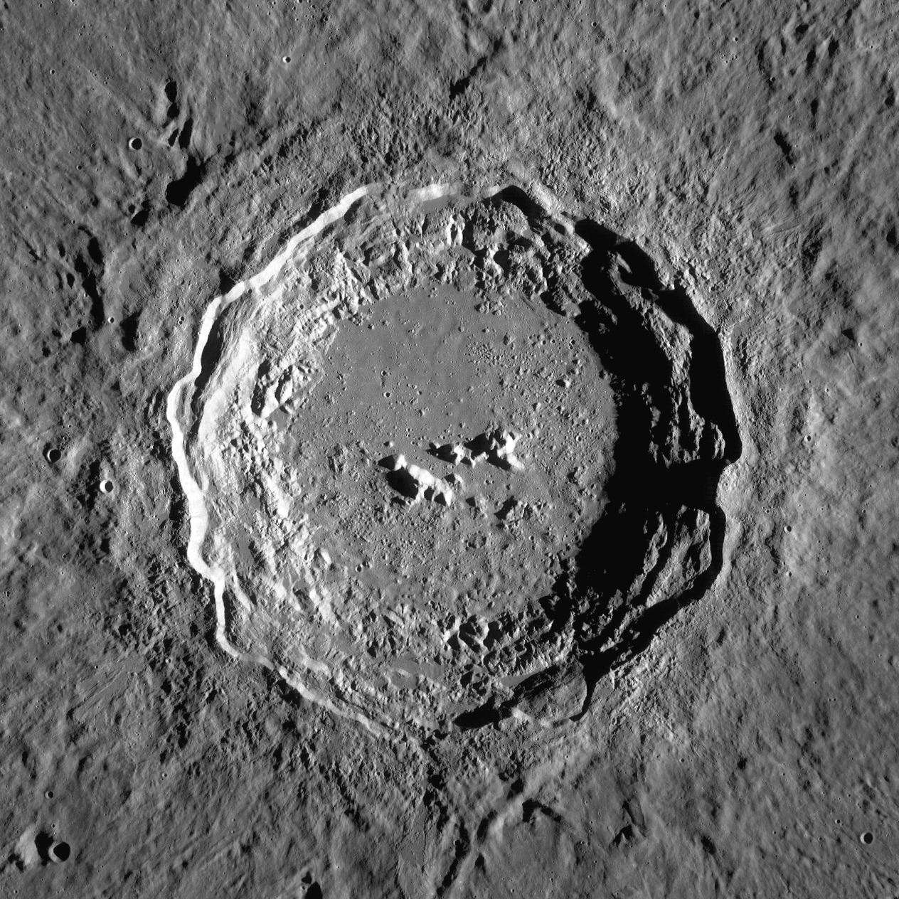
Courtesy of Wikipedia, the pictures below are the Copernicus crater on the Moon as well as an indicator of its location on the Moon. It is visible with binoculars.
The diameter of the crater is 93 km. Since the Moon is 384,400 km from Earth, that means the angle subtended by the crater, as viewed from the Earth, is about
.
So how much is 43″ of arc per century? That’s about the speed as, hypothetically, pointing at the left edge of this lunar crater (which cannot be seen by the naked eye) and then slowly moving your figure so that, about 115 years later, your finger is pointing at the right edge of the crater.
Said another way, the diameter of the Moon is about 3475 km, so that the angle subtended by the Moon, as viewed from the Earth, is about
.
So, at the rate of per century, it would take centuries, or about 43,000 years, to trace the angle subtended by the moon.
Needless to say, 43” of arc per century is really, really slow.
Nevertheless, and remarkably, this itty, bitty precession was observable by careful 19th century astronomers with the telescopes that were available then. At the time, this precession was the great unsolved mystery of Newtonian physics that was only answered after two generations later with the discovery of general relativity.
Lately, for my own leisure reading, I’ve been enjoying the murder-mystery novels of Dorothy Sayers. Her books are an enjoyable trip back in time, as she paints a very vivid portrait of English life of during the interwar years of the 1920s and 1930s. (Of course, at the time she was writing, no one had any idea that the Great War would not actually be the war to end all wars, as was the popular sentiment of the time.) Indeed, her first novel was published literally a century ago in 1923. The lead character, Lord Peter Wimsey (back then, the aristocracy was still part of English culture), has a distinctive way of speaking that makes the novels so delightful. A hallmark of the Sayers novels is that she didn’t merely write whodunit stories; instead, she strove to write novels in which a detective story happens to happen.
As an aside, I learned in her novel Gaudy Night that the adjective Oxonian means “related to Oxford,” which led me to further learn that my hometown of Oxon Hill, Maryland was so named because somebody, centuries ago, thought that the landscape of that part of the state reminded him of Oxford, England. While that comparison might have been reasonable centuries ago, it certainly would raise eyebrows today.
Anyway, with all that as background, in her story Unnatural Death, the following figure depicts an aerial view of a witness’s testimony at a key point in the story. I think I can describe this much of the scene without giving away the plot: the witnesses stood just inside the door of elderly Miss Dawson’s bedroom. A screen blocked direct observation of Miss Dawson as she lay in bed, but the witnesses could see Miss Dawson in the mirror.
As I read the novel, I immediately noticed that the mirror in the figure was not a perfect reflector… at the mirror, the angles of reflection of the dashed path of light are quite different. Indeed, I pulled out my protractor: the angle where the word “Mirror” is located has a measure of about 52 degrees, while the opposite reflected angle has a measure of about 72 degrees.
As this is was part of a murder-mystery novel, I thought: what could be the cause of this disparity? To be a good detective, any explanation, no matter how implausible, must be thought of and reasoned out.
One explanation of the different angles is that, somehow, the speed of light changed in the room. This is the same principle behind Snell’s Law, which explains the refraction of light as it travels between air and water. Since the speed of light in air () is different than the speed of light in water (), the angle of incidence ( is different from the angle of refraction (), but they are related through the formula
.
This relationship occurs because of Fermat’s principle, which says that light always travels in a path that requires the least amount of time. Ordinarily, this means that light travels in a straight line. However, if the speed of light should change (say, when traveling through both air and water), then the path of the light is refracted.
Fermat’s principle also explains why light reflects at equal angles if the speed of light is constant (as amusingly illustrated in this PBS video by Dianna Cowern, a.k.a. Physics Girl). However, if the speed of light should somehow change in the room at the point where the light reflects, then the light would bounce at a different angle for the same reason that Snell’s Law works.
In this case, the angles and are complementary to the 52-degree and 72-degree angles, respectively. By the cofunction trigonometric identities, this means that
and ,
so that Snell’s Law can be rewritten as
.
In other words, one explanation for the unusual path of light is that the speed of light was almost exactly twice as fast in one part of room than in the other part… and the exact threshold of this change occurred at the point where the light hit the mirror. Perhaps there was some kind of fog, mist, or other contaminant in the air near poor Miss Dawson that was so thick that light slowed to half its usual speed. So that’s one explanation.
The other explanation, of course, is that the artist who drew the picture just did a lousy job depicting the reflected light.
As this was part of a murder-mystery, both options are still open to investigation. (Yes, that was tongue-in-cheek.)
For what it’s worth, the figure in my book was not exactly the same as Sayers’ original drawing — clearly, modern word processing was used that was unavailable in the 1930s. One of these days, I may visit the Wade Center in Wheaton, Illinois, which has an impressive collection of Sayers’ works, to peruse a first-run printing of Unnatural Death to see if the figure in my book is faithful to the one that appeared when the novel was first published.


![= \displaystyle \frac{\ell}{mr^2} \frac{d}{d\theta} \left[ \frac{dr}{dt} \right]](https://s0.wp.com/latex.php?latex=%3D+%5Cdisplaystyle+%5Cfrac%7B%5Cell%7D%7Bmr%5E2%7D+%5Cfrac%7Bd%7D%7Bd%5Ctheta%7D+%5Cleft%5B+%5Cfrac%7Bdr%7D%7Bdt%7D+%5Cright%5D&bg=ffffff&fg=000000&s=0&c=20201002)
![= \displaystyle \frac{\ell}{mr^2} \frac{d}{d\theta} \left[ - \frac{\ell}{m} \frac{d}{d\theta} \left( \frac{1}{r} \right) \right]](https://s0.wp.com/latex.php?latex=%3D+%5Cdisplaystyle+%5Cfrac%7B%5Cell%7D%7Bmr%5E2%7D+%5Cfrac%7Bd%7D%7Bd%5Ctheta%7D+%5Cleft%5B+-+%5Cfrac%7B%5Cell%7D%7Bm%7D+%5Cfrac%7Bd%7D%7Bd%5Ctheta%7D+%5Cleft%28+%5Cfrac%7B1%7D%7Br%7D+%5Cright%29+%5Cright%5D&bg=ffffff&fg=000000&s=0&c=20201002)
![= \displaystyle - \frac{\ell^2}{m^2r^2} \frac{d}{d\theta} \left[ \frac{d}{d\theta} \left( \frac{1}{r} \right) \right]](https://s0.wp.com/latex.php?latex=%3D+%5Cdisplaystyle+-+%5Cfrac%7B%5Cell%5E2%7D%7Bm%5E2r%5E2%7D+%5Cfrac%7Bd%7D%7Bd%5Ctheta%7D+%5Cleft%5B+%5Cfrac%7Bd%7D%7Bd%5Ctheta%7D+%5Cleft%28+%5Cfrac%7B1%7D%7Br%7D+%5Cright%29+%5Cright%5D&bg=ffffff&fg=000000&s=0&c=20201002)

 .
. using the quadratic formula; more on that later.) To apply the method of successive approximation, we will rewrite this so that
  , or
, or .
. .
. .
. .
. . Then


 into a calculator, then entering
  , and then repeatedly hitting the
  button.
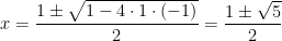 .
. .
. . Unfortunately, if we start with a guess near this root, like
  , the sequence unexpectedly diverges from
  but eventually converges to the positive root
  :
:


 north,
  west, which is about 40 miles NNW of Spokane. (Images made by

 north,
  west — which is indeed in Spokane — and then misconverted from decimal notation to minutes and seconds.

 . Furthermore, if
  , then this represents an ellipse with eccentricity
  whose major axis lies on the
  axis, with one focus located at the origin.
 . Under this assumption,
  and
and  , so let me rewrite the previous equation in terms of
  :
:
 ,
,
 from the center to the foci satisfies
 ,
,


 , this means that the origin is, once again, one of the foci of the hyperbola.
 of the hyperbola is easily computed as
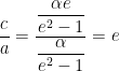 ,
,

 . With this substitution, the equation in rectangular coordinates simplifies to
 .
. , so that
  . Then the equation in rectangular coordinates simplifies to

 .
. ,
, to the left of the vertex. In other words, the origin is the focus of the parabola. (For what it’s worth, the directrix of the parabola would be the vertical line
  , located
  to the right of the vertex.)
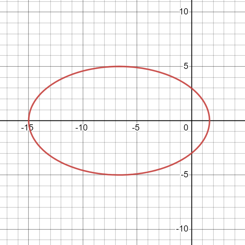
 .
.


 so that
 .
. ,
, ,
, ,
, .
. ,
,


 . Therefore, since the foci of the ellipse are distance
  , or
, or  . That is, the origin is one focus of the ellipse. (For the little it’s worth, the other focus is located at
  .
. .
. and
and  . For this ellipse, the planet’s closest approach to the Sun occurs at
  :
: ,
, :
: .
. of the major axis of the ellipse is the sum of these two distances:

 .
. , we can also compute


 using
using  . The reason for choosing the letter
  and
and  and altering the value of
  . So, not surprisingly, increasing
 and
and  , so the distance from the origin is the same for all angles. However, as
 and
and  . In particular, the denominator is always positive. Therefore, the value of
  . So, for example, when
  is as close as the graph gets to the origin. Let’s call this closest distance
  ; in the context of a planet’s orbit around the sun, this represent perihelion. Then we have
  .
. , the graph switches from an ellipse to a parabola, where the origin is the focus of the parabola. For
  , the graph becomes a hyperbola. However, since we’re mostly going to be concerned with stable planetary orbits in this series, we won’t dwell too much on the case
  .
. , and then alter the value of
 . If I had changed the upper bound to something larger than
  , the spiral would continue.
 is a multiple of
  , or
, or  . If
. If  , then the angle of closest approach to the origin would
  , and the graph simply cycles over itself. However, if
  , then this angle
  .
. . Therefore, the amount of precession would be
  radians
  . Therefore, after 19 “leafs” of the spiral, the graph would begin to cycle on top of itself.
 ,
, ,
, .
. is equal to
  .
. is the gravitational constant of the universe.
 is the mass of the Sun.
 is the mass of the planet.
 ,
, .
. .
. and
and  . The number
  is the eccentricity of the ellipse, while
  is proportional to the size of the ellipse.
![u''(\theta) + u(\theta) = \displaystyle \frac{GMm^2}{\ell^2} + \frac{3GM}{c^2} [u(\theta)]^2](https://s0.wp.com/latex.php?latex=u%27%27%28%5Ctheta%29+%2B+u%28%5Ctheta%29+%3D+%5Cdisplaystyle+%5Cfrac%7BGMm%5E2%7D%7B%5Cell%5E2%7D+%2B+%5Cfrac%7B3GM%7D%7Bc%5E2%7D+%5Bu%28%5Ctheta%29%5D%5E2&bg=ffffff&fg=000000&s=0&c=20201002) ,
,
![\approx \displaystyle \frac{1}{\alpha} \left[1 + \epsilon \cos \left(\theta - \frac{\delta \theta}{\alpha} \right) \right]](https://s0.wp.com/latex.php?latex=%5Capprox+%5Cdisplaystyle+%5Cfrac%7B1%7D%7B%5Calpha%7D+%5Cleft%5B1+%2B+%5Cepsilon+%5Ccos+%5Cleft%28%5Ctheta+-+%5Cfrac%7B%5Cdelta+%5Ctheta%7D%7B%5Calpha%7D+%5Cright%29+%5Cright%5D&bg=ffffff&fg=000000&s=0&c=20201002) .
. radians per orbit
 radians per orbit,
 . After nine orbits, the planet returns to its original position. Suppose, for the sake of argument, that each orbit of the planet depicted in the figure is four months, or one third of Earth’s year. Then the amount of precession would be
  per four months, or
  per year, or
  per century.
 is equal to 60′ (minutes) of arc and each 1′ is equal to 60″ (seconds) of arc, that means 1″ of arc is the same as
  , so that 43″ of arc per century is about
  per century. That’s about a million times smaller than the precession of the fictitious planet in the above figure.
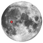
 .
. .
. centuries, or about 43,000 years, to trace the angle subtended by the moon.
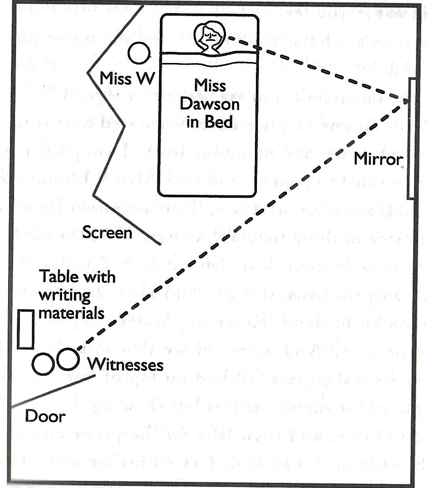
 ) is different than the speed of light in water (
 ), the angle of incidence (
 is different from the angle of refraction (
 ), but they are related through the formula
 .
. and
and  and
and  ,
, .
.