In this series, I’m discussing how ideas from calculus and precalculus (with a touch of differential equations) can predict the precession in Mercury’s orbit and thus confirm Einstein’s theory of general relativity. The origins of this series came from a class project that I assigned to my Differential Equations students maybe 20 years ago.
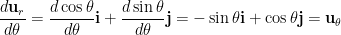
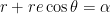
We previously showed that if the motion of a planet around the Sun is expressed in polar coordinates 
where 


the second equation arises since

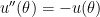
We now take the perspective of a student who is taking a first-semester course in differential equations. There are two standard techniques for solving a second-order non-homogeneous differential equations with constant coefficients. One of these is the method of undetermined coefficients. First, we solve the associated homogeneous differential equation
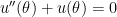
The characteristic equation of this differential equation is 

(As an aside, this is one answer to the common question, “What are complex numbers good for?” The answer is naturally above the heads of Algebra II students when they first encounter the mysterious number 
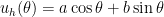
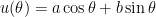
Next, we find a particular solution to the original differential equation. Since the right-hand side is a constant and 


Clearly, 


Therefore, 
Next, the general solution of the nonhomogeneous differential equation is found by adding the general solution to the associated homogeneous differential equation and the particular solution:
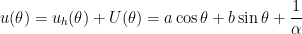
Finally, to determine 


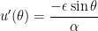
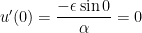
From the second initial condition,


From these two constants, we obtain

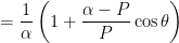

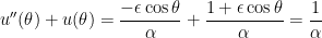
where 
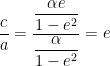
Finally, since 
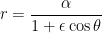
so that, as shown earlier in this series, the orbit is an ellipse with eccentricity 
The reader will notice that this solution is pretty much a carbon-copy of the previous post. The difference is that calculus students wouldn’t necessarily be able to independently generate the solutions of the associated homogeneous differential equation and a particular solution of the nonhomogeneous differential equation, and so the line of questioning is designed to steer students toward the answer.

 .
. and
and  .
. and
and  work. Once that conceptual barrier is broken, they’ll usually produce the solutions
  and
and  .
. also solves the associated homogeneous differential equation.
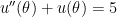 . Can you think of an easy function that’s a solution?
 is a constant function, then clearly
  and
and  , so that
  works.
 is a solution of
  is a solution of
  will work.
 :
: and then substitute
  , with the Sun at the origin, then under Newtonian mechanics (i.e., without general relativity) the motion of the planet follows the differential equation
  . Since
  is the reciprocal of
  is extremely unlikely, this means that the planet orbits the Sun in an ellipse, with the Sun at one focus of the ellipse.
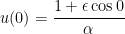


 .
.
 .
. :
: ,
, ,
, ,
, and the acceleration
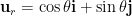
  are vectors. When written in polar coordinates, this becomes
![{\bf F} = m \displaystyle \left[ \frac{d^2r}{dt^2} - r \left( \frac{d\theta}{dt} \right)^2 \right] {\bf u}_r + m \left(r \frac{d^2 \theta}{d t^2} + 2 \frac{dr}{dt} \frac{d\theta}{dt} \right) {\bf u}_\theta](https://s0.wp.com/latex.php?latex=%7B%5Cbf+F%7D+%3D+m+%5Cdisplaystyle+%5Cleft%5B+%5Cfrac%7Bd%5E2r%7D%7Bdt%5E2%7D+-+r+%5Cleft%28+%5Cfrac%7Bd%5Ctheta%7D%7Bdt%7D+%5Cright%29%5E2+%5Cright%5D+%7B%5Cbf+u%7D_r+%2B+m+%5Cleft%28r+%5Cfrac%7Bd%5E2+%5Ctheta%7D%7Bd+t%5E2%7D+%2B+2+%5Cfrac%7Bdr%7D%7Bdt%7D+%5Cfrac%7Bd%5Ctheta%7D%7Bdt%7D+%5Cright%29+%7B%5Cbf+u%7D_%5Ctheta&bg=ffffff&fg=000000&s=0&c=20201002) ,
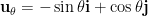
, is a unit vector pointing away from the origin and
  is a unit vector perpendicular to
  .
. ,
, is the mass of the sun,
  is the mass of the planet, and
  is the gravitational constant of the universe (which is a constant, no matter what
 ![m \displaystyle \left[ \frac{d^2r}{dt^2} - r \left( \frac{d\theta}{dt} \right)^2 \right] = \displaystyle -\frac{GMm}{r^2}](https://s0.wp.com/latex.php?latex=m+%5Cdisplaystyle+%5Cleft%5B+%5Cfrac%7Bd%5E2r%7D%7Bdt%5E2%7D+-+r+%5Cleft%28+%5Cfrac%7Bd%5Ctheta%7D%7Bdt%7D+%5Cright%29%5E2+%5Cright%5D+%3D+%5Cdisplaystyle+-%5Cfrac%7BGMm%7D%7Br%5E2%7D&bg=ffffff&fg=000000&s=0&c=20201002) ,
, .
. ,
, is a constant, and
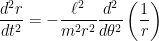 .
.


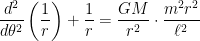
![\displaystyle \frac{\ell^2}{m^2 r^2} \left[ \frac{d^2}{d\theta^2} \left( \frac{1}{r} \right) + \frac{1}{r} \right] = \displaystyle \frac{GM}{r^2}](https://s0.wp.com/latex.php?latex=%5Cdisplaystyle++%5Cfrac%7B%5Cell%5E2%7D%7Bm%5E2+r%5E2%7D+%5Cleft%5B+%5Cfrac%7Bd%5E2%7D%7Bd%5Ctheta%5E2%7D+%5Cleft%28+%5Cfrac%7B1%7D%7Br%7D+%5Cright%29+%2B+%5Cfrac%7B1%7D%7Br%7D+%5Cright%5D++%3D+%5Cdisplaystyle+%5Cfrac%7BGM%7D%7Br%5E2%7D&bg=ffffff&fg=000000&s=0&c=20201002)
 .
. , we finally obtain the governing equation
 .
. as the constant on the right-hand side instead of just
  ,
, ,
, and
and  directors are
  and
and  , and the unit vectors
  and
and  are perpendicular, pointing in the positive
  and positive
  directions.
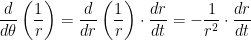
 . This may be rewritten as
 ,
,
 .
.
 .
. .
. .
. , or a distance
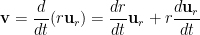

 .
.

![= \displaystyle \left[ \frac{d^2r}{dt^2} - r \left(\frac{d\theta}{dt} \right)^2 \right] {\bf u}_r + \left[ 2\frac{dr}{dt} \frac{d\theta}{dt} + r \frac{d^2\theta}{dt^2} \right] {\bf u}_\theta](https://s0.wp.com/latex.php?latex=%3D+%5Cdisplaystyle+%5Cleft%5B+%5Cfrac%7Bd%5E2r%7D%7Bdt%5E2%7D+-++r+%5Cleft%28%5Cfrac%7Bd%5Ctheta%7D%7Bdt%7D+%5Cright%29%5E2+%5Cright%5D+%7B%5Cbf+u%7D_r+%2B+%5Cleft%5B+2%5Cfrac%7Bdr%7D%7Bdt%7D+%5Cfrac%7Bd%5Ctheta%7D%7Bdt%7D+%2B+r+%5Cfrac%7Bd%5E2%5Ctheta%7D%7Bdt%5E2%7D+%5Cright%5D+%7B%5Cbf+u%7D_%5Ctheta&bg=ffffff&fg=000000&s=0&c=20201002) .
. ,
, ;
; in a form that depends only on


 .
. .
.


![= \displaystyle \frac{\ell}{mr^2} \frac{d}{d\theta} \left[ \frac{dr}{dt} \right]](https://s0.wp.com/latex.php?latex=%3D+%5Cdisplaystyle+%5Cfrac%7B%5Cell%7D%7Bmr%5E2%7D+%5Cfrac%7Bd%7D%7Bd%5Ctheta%7D+%5Cleft%5B+%5Cfrac%7Bdr%7D%7Bdt%7D+%5Cright%5D&bg=ffffff&fg=000000&s=0&c=20201002)
![= \displaystyle \frac{\ell}{mr^2} \frac{d}{d\theta} \left[ - \frac{\ell}{m} \frac{d}{d\theta} \left( \frac{1}{r} \right) \right]](https://s0.wp.com/latex.php?latex=%3D+%5Cdisplaystyle+%5Cfrac%7B%5Cell%7D%7Bmr%5E2%7D+%5Cfrac%7Bd%7D%7Bd%5Ctheta%7D+%5Cleft%5B+-+%5Cfrac%7B%5Cell%7D%7Bm%7D+%5Cfrac%7Bd%7D%7Bd%5Ctheta%7D+%5Cleft%28+%5Cfrac%7B1%7D%7Br%7D+%5Cright%29+%5Cright%5D&bg=ffffff&fg=000000&s=0&c=20201002)
![= \displaystyle - \frac{\ell^2}{m^2r^2} \frac{d}{d\theta} \left[ \frac{d}{d\theta} \left( \frac{1}{r} \right) \right]](https://s0.wp.com/latex.php?latex=%3D+%5Cdisplaystyle+-+%5Cfrac%7B%5Cell%5E2%7D%7Bm%5E2r%5E2%7D+%5Cfrac%7Bd%7D%7Bd%5Ctheta%7D+%5Cleft%5B+%5Cfrac%7Bd%7D%7Bd%5Ctheta%7D+%5Cleft%28+%5Cfrac%7B1%7D%7Br%7D+%5Cright%29+%5Cright%5D&bg=ffffff&fg=000000&s=0&c=20201002)
 .
. .
. , or
, or .
. .
. .
. .
. . Then
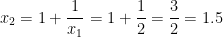


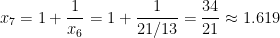
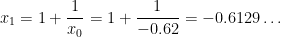
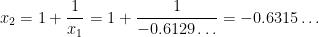
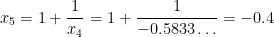
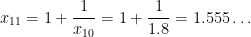
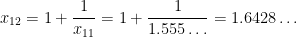
 into a calculator, then entering
  , and then repeatedly hitting the
  button.
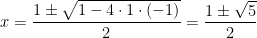 .
. .
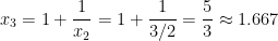
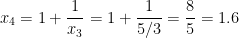
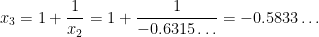
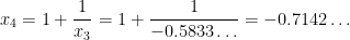
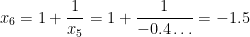
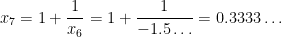
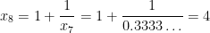
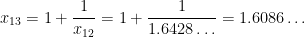
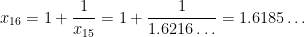
. . Unfortunately, if we start with a guess near this root, like
  , the sequence unexpectedly diverges from
  but eventually converges to the positive root
  :
:


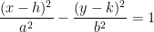
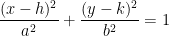
 . Furthermore, if
  , then this represents an ellipse with eccentricity
  whose major axis lies on the
  . Under this assumption,
  and
and  , so let me rewrite the previous equation in terms of
  :
:
 ,
,
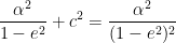
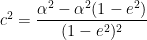
 from the center to the foci satisfies
 ,
,


 , this means that the origin is, once again, one of the foci of the hyperbola.
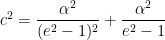
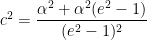
 of the hyperbola is easily computed as
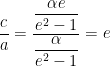 ,
,

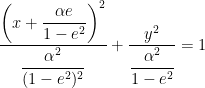
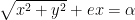
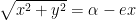
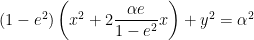
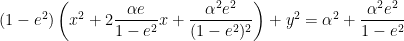
 . With this substitution, the equation in rectangular coordinates simplifies to
 .
. , so that
  . Then the equation in rectangular coordinates simplifies to

 .
. ,
, to the left of the vertex. In other words, the origin is the focus of the parabola. (For what it’s worth, the directrix of the parabola would be the vertical line
  , located
  to the right of the vertex.)
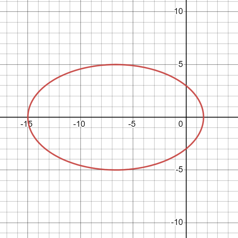
 .
.


 so that
 .
. ,
, ,
, ,
, .
. ,
,


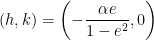
 . Therefore, since the foci of the ellipse are distance
  , or
, or  . That is, the origin is one focus of the ellipse. (For the little it’s worth, the other focus is located at
  .
. .
.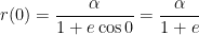 ,
, :
: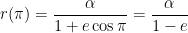 .
. of the major axis of the ellipse is the sum of these two distances:
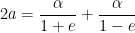

 .
. , we can also compute