In a recent class with my future secondary math teachers, we had a fascinating discussion concerning how a teacher should respond to the following question from a student:
Is it ever possible to prove a statement or theorem by proving a special case of the statement or theorem?
Usually, the answer is no. In this series of posts, we’ve seen that a conjecture could be true for the first 40 cases or even the first  cases yet not always be true. We’ve also explored the computational evidence for various unsolved problems in mathematics, noting that even this very strong computational evidence, by itself, does not provide a proof for all possible cases.
However, there are plenty of examples in mathematics where it is possible to prove a theorem by first proving a special case of the theorem. For the remainder of this series, I’d like to list, in no particular order, some common theorems used in secondary mathematics which are typically proved by first proving a special case.
The following problem appeared on a homework assignment of mine about 30 years ago when I was taking Honors Calculus out of Apostol’s book. I still remember trying to prove this theorem (at the time, very unsuccessfully) like it was yesterday.
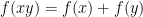
Theorem. If  is a continuous function so that
  , then
  for some constant
  .
.
Proof. The proof mirrors that of the uniqueness of the logarithm function, slowly proving special cases to eventually prove the theorem for all real numbers  .
.
Case 1.  . If we set
  and
and  , then


Case 2.  . If is a positive integer, then


 .
.
(Technically, this should be proven by induction, but I’ll skip that for brevity.) If we let  , then .
Case 3.  . If is a negative integer, let
  , where
  is a positive integer. Then


Case 4.  . If is a rational number, then write
  , where
  and
and  are integers and is a positive integer. We’ll use the fact that
  , where the sum is repeated times.


Case 5.  . If is a real number, then let
  be a sequence of rational numbers that converges to , so that

Then, since  is continuous,


QED

Random Thought #1: The continuity of the function was only used in Case 5 of the above proof. I’m nearly certain that there’s a pathological discontinuous function that satisfies which is not the function . However, I don’t know what that function might be.
Random Thought #2: For what it’s worth, this same idea can be used to solve the following problem that was posed during UNT’s Problem of the Month competition in January 2015. I won’t solve the problem here so that my readers can have the fun of trying to solve it for themselves.
Problem. Determine all nonnegative continuous functions that satisfy
 .
.
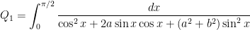
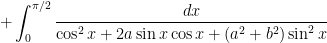
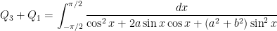
 So far in this series, I’ve shown that


 . This is permissible because
  — which is why I needed to adjust the limits of integration in the first place. I obtain


 ,
, ,
,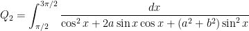 ,
, .
. and apply the substitution
  , or
, or  . Then
  , and the endpoints change from
  to
to  . Therefore,
 .
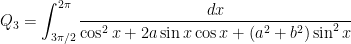
. and
and  — to rewrite
 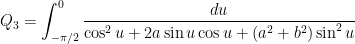 .
. back to
  .
. into a single integral:
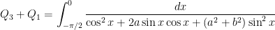
 . We use the substitution
  , or
, or  , so that
 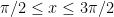 to
to  , so that
 .
. ,
, ,
,

 , and so

 , partial fractions, and even contour integration and residues.
![[a,b]](https://s0.wp.com/latex.php?latex=%5Ba%2Cb%5D&bg=ffffff&fg=000000&s=0&c=20201002) which is differentiable on the interior
which is differentiable on the interior  , then there is a point
  so that
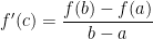

 and
and  , then there is a point
  .
.
 ,
,
 satisfies the hypotheses of Rolle’s Theorem and conclude that there must be a point so that
  , from which we obtain the conclusion of the Mean Value Theorem.
 , we have
  .
. .
.
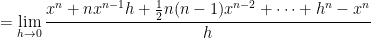
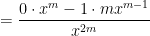
![= \displaystyle \lim_{h \to 0} \left[ n x^{n-1} + \frac{1}{2} n(n-1) x^{n-2} h + \dots + h^{n-1} \right]](https://s0.wp.com/latex.php?latex=%3D+%5Cdisplaystyle+%5Clim_%7Bh+%5Cto+0%7D+%5Cleft%5B+n+x%5E%7Bn-1%7D+%2B+%5Cfrac%7B1%7D%7B2%7D+n%28n-1%29+x%5E%7Bn-2%7D+h+%2B+%5Cdots+%2B+h%5E%7Bn-1%7D+%5Cright%5D&bg=ffffff&fg=000000&s=0&c=20201002)


 , then the theorem is trivially true since
  , and the derivative of a constant is zero.
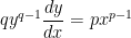
 , where
  is a positive integer. Then, using the Quotient Rule,


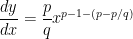
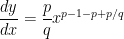
 , where
  . Then:
![y^q = \displaystyle \left[ x^{p/q} \right]^q](https://s0.wp.com/latex.php?latex=y%5Eq+%3D+%5Cdisplaystyle+%5Cleft%5B+x%5E%7Bp%2Fq%7D+%5Cright%5D%5Eq&bg=ffffff&fg=000000&s=0&c=20201002)


![\displaystyle \frac{dy}{dx} = \displaystyle \frac{p}{q} \frac{x^{p-1}}{[x^{p/q}]^{q-1}}](https://s0.wp.com/latex.php?latex=%5Cdisplaystyle+%5Cfrac%7Bdy%7D%7Bdx%7D+%3D+%5Cdisplaystyle+%5Cfrac%7Bp%7D%7Bq%7D+%5Cfrac%7Bx%5E%7Bp-1%7D%7D%7B%5Bx%5E%7Bp%2Fq%7D%5D%5E%7Bq-1%7D%7D&bg=ffffff&fg=000000&s=0&c=20201002)


 .
. . Suppose that
  has the following four properties:

 for all
 for all
  .
.