Last summer, Math With Bad Drawings had a nice series on the notion of infinity that I recommend highly. This topic is a perennial struggle for math majors to grasp, and I like the approach that the author uses to sell this difficult notion.
Here’s Part 2 on the harmonic series, which is extremely well-written and which I recommend highly. Here’s a brief summary: the infinite harmonic series

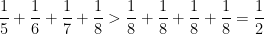
diverges. However, if you eliminate from the harmonic series all of the fractions whose denominator contains a 9, then the new series converges! This series has been called the Kempner series, named after the mathematician who first published this result about 100 years ago.

Source: http://smbc-comics.com/index.php?id=3777
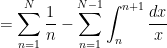
To prove this, we’ll examine the series whose denominators are between 1 and 8, between 10 and 88, between 100 and 888, etc. First, each of the terms in the partial sum
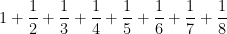
is less than or equal to  , and so the sum of the above eight terms must be less than
  .
.
Next, each of the terms in the sum
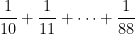
is less than  . Notice that there are
  terms in this sum since there are 8 possibilities for the first digit of the denominator (1 through 8) and 9 possibilities for the second digit (0 through 8). So the sum of these 72 terms must be less than
  .
.
Next, each of the terms in the sum
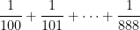
is less than  . Notice that there are
  terms in this sum since there are 8 possibilities for the first digit of the denominator (1 through 8) and 9 possibilities for the second and third digits (0 through 8). So the sum of these terms must be less than
  .
.
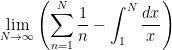
Continuing, we see that the Kempner series is bounded above by

Using the formula for an infinite geometric series, we see that the Kempner series converges, and the sum of the Kempner series must be less than  .
.
Using the same type of reasoning, much sharper bounds for the sum of the Kempner series can also be found. This 100-year-old article from the American Mathematical Monthly demonstrates that the sum of the Kempner series is between  and
and  . For more information about approximating the sum of the Kempner series, see Mathworld and Wikipedia.
It should be noted that there’s nothing particularly special about the number  in the above discussion. If all denominators containing
  , or any finite pattern, are eliminated from the harmonic series, then the resulting series will always converge.


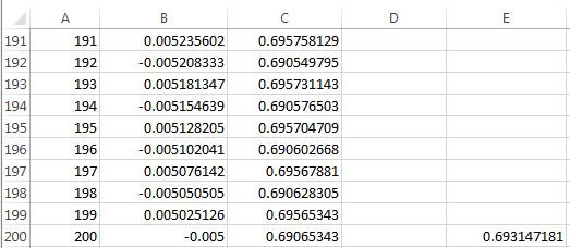


 We see that, as expected, the partial sums are converging to
 ,
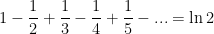
, converges conditionally and not absolutely.
 , the
, the  th partial sum of
  converges. Furthermore, the limit of any subsequence, like
  , must also converge to
  and
and  is an integer, then


 .
. ,
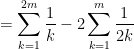
,![s_{2m} = \ln(2m) - \ln 1 + \displaystyle \left( \sum_{k=1}^{2m} \frac{1}{k} - [\ln(2m) - \ln 1]\right)](https://s0.wp.com/latex.php?latex=s_%7B2m%7D+%3D+%5Cln%282m%29+-+%5Cln+1+%2B+%5Cdisplaystyle+%5Cleft%28+%5Csum_%7Bk%3D1%7D%5E%7B2m%7D+%5Cfrac%7B1%7D%7Bk%7D+-+%5B%5Cln%282m%29+-+%5Cln+1%5D%5Cright%29&bg=ffffff&fg=000000&s=0&c=20201002)
![- [\ln m - \ln 1] - \displaystyle \left( \sum_{k=1}^m \frac{1}{k} - [\ln m - \ln 1]\right)](https://s0.wp.com/latex.php?latex=-+%5B%5Cln+m+-+%5Cln+1%5D+-+%5Cdisplaystyle+%5Cleft%28+%5Csum_%7Bk%3D1%7D%5Em+%5Cfrac%7B1%7D%7Bk%7D+-+%5B%5Cln+m+-+%5Cln+1%5D%5Cright%29&bg=ffffff&fg=000000&s=0&c=20201002) .
. and
and  , we have
 .
. :
: .
.
 ,
, .
. ,
, .
. ,
,  ,
,  , and
, and  . In sixth place (a distant sixth place) is probably
  , the Euler-Mascheroni constant. See
  by
by
 .
. is clearly decreasing for
  , and so the maximum value of
  on the interval
 ![[n,n+1]](https://s0.wp.com/latex.php?latex=%5Bn%2Cn%2B1%5D&bg=ffffff&fg=000000&s=0&c=20201002) must occur at the left endpoint, while the minimum value must occur at the right endpoint. Since the length of this interval is
must occur at the left endpoint, while the minimum value must occur at the right endpoint. Since the length of this interval is  ,
, .
. clearly decreases to
 .
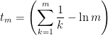
. , where
  and
and  is an integer. Then by separating the even and odd terms, we obtain

 .
. .
.

 converges conditionally if it converges to a finite number but
  diverges. Indeed, by suitably rearranging the terms, the sum can be changed so that the (rearranged) series converges to any finite value. Even worse, the terms can be rearranged so that the sum converges to either
  or
or  . (Of course, this can’t happen for finite sums, and rearrangements of an absolutely convergent series do not change the value of the sum.)
 :
:
 but each factor on the right-hand side is less than 1. The error, of course, stems from conditional convergence (the terms in the top product cannot be rearranged).
 ,
, ,
, ,
, ,
,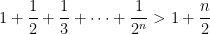 .
. , we can conclude that the harmonic series diverges.

 and
and  , there is an alternative answer:
 .
.
 .
. over an interval that contains neither
  or
or  , then either
  or
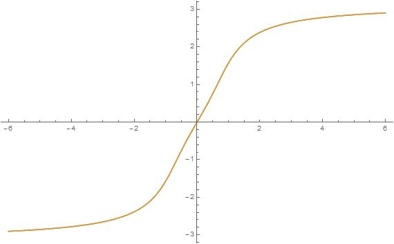
or  can be used. Courtesy of Mathematica:
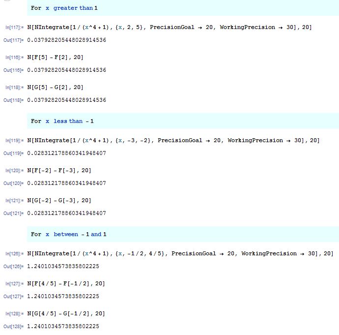

 (or both), then only using
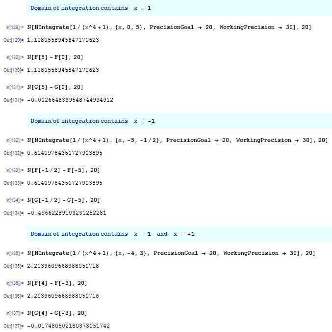
 that appeared several posts ago ultimately makes a big difference in the final answers that are obtained.
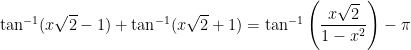 if
if  ,
, if
if  ,
, if
if  ,
, and
and  are the unique values so that
 ,
, .
. and
and  . Indeed, it’s apparent that these have to be the two transition points because these are the points where
  is undefined. However, it would be more convincing to show this directly.
 .
.
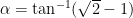 and
and  , so that
 ,
, .
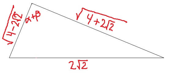
. and
and  can be represented in the figure below:
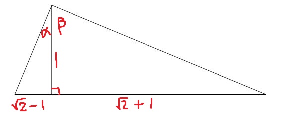
 . I will use the Pythagorean theorem to find the lengths of the other two sides. For the small right triangle containing

 ,
, .
. . In other words,
  is an odd function using the fact that
  is also an odd function:
![= \tan^{-1} ( -[x\sqrt{2} + 1] ) + \tan^{-1}( -[x \sqrt{2} - 1])](https://s0.wp.com/latex.php?latex=%3D+%5Ctan%5E%7B-1%7D+%28+-%5Bx%5Csqrt%7B2%7D+%2B+1%5D+%29+%2B+%5Ctan%5E%7B-1%7D%28+-%5Bx+%5Csqrt%7B2%7D+-+1%5D%29&bg=ffffff&fg=000000&s=0&c=20201002)

![= - \left[ \tan^{-1} ( x\sqrt{2} + 1 ) + \tan^{-1}( x \sqrt{2} - 1) \right]](https://s0.wp.com/latex.php?latex=%3D+-+%5Cleft%5B+%5Ctan%5E%7B-1%7D+%28+x%5Csqrt%7B2%7D+%2B+1+%29+%2B+%5Ctan%5E%7B-1%7D%28+x+%5Csqrt%7B2%7D+-+1%29+%5Cright%5D&bg=ffffff&fg=000000&s=0&c=20201002)
 .
. , and so
  ,
, ,
, .
. and
and  :
:
 and
and  ,
, ,
, .
. ,
, and
and  must differ if
  is in the interval
 ![[-\pi,-\pi/2]](https://s0.wp.com/latex.php?latex=%5B-%5Cpi%2C-%5Cpi%2F2%5D&bg=ffffff&fg=000000&s=0&c=20201002) or in the interval
or in the interval ![[\pi/2,\pi]](https://s0.wp.com/latex.php?latex=%5B%5Cpi%2F2%2C%5Cpi%5D&bg=ffffff&fg=000000&s=0&c=20201002) .
. ,
, .
. , namely
  where this happens, I also note that
  ,
,  , and
, and  are increasing functions, and so
  . Likewise, to determine where
  .
.
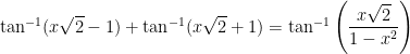
 and
and  , I obtain
![\tan \left[ \tan^{-1} ( x\sqrt{2} - 1 ) + \tan^{-1}( x \sqrt{2} + 1) \right] = \displaystyle \frac{x \sqrt{2} - 1 + x \sqrt{2} + 1}{1 - (x\sqrt{2} - 1)(x\sqrt{2} + 1)}](https://s0.wp.com/latex.php?latex=%5Ctan+%5Cleft%5B+%5Ctan%5E%7B-1%7D+%28+x%5Csqrt%7B2%7D+-+1+%29+%2B+%5Ctan%5E%7B-1%7D%28+x+%5Csqrt%7B2%7D+%2B+1%29+%5Cright%5D+%3D+%5Cdisplaystyle+%5Cfrac%7Bx+%5Csqrt%7B2%7D+-+1+%2B+x+%5Csqrt%7B2%7D+%2B+1%7D%7B1+-+%28x%5Csqrt%7B2%7D+-+1%29%28x%5Csqrt%7B2%7D+%2B+1%29%7D&bg=ffffff&fg=000000&s=0&c=20201002)


 .
.
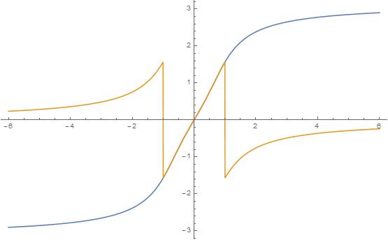
 and
and  have different graphs. (The vertical lines in the orange graph indicate where the right-hand side is undefined when
  :
: