In my capstone class for future secondary math teachers, I ask my students to come up with ideas for engaging their students with different topics in the secondary mathematics curriculum. In other words, the point of the assignment was not to devise a full-blown lesson plan on this topic. Instead, I asked my students to think about three different ways of getting their students interested in the topic in the first place.
I plan to share some of the best of these ideas on this blog (after asking my students’ permission, of course).
This student submission comes from my former student Michelle McKay. Her topic, from Algebra II: deriving the distance formula.

C. How has this topic appeared in pop culture?
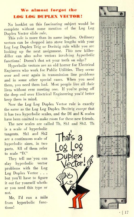
Numb3rs is a relatively popular TV show that revolves around the character Dr. Charlie Eppes, a mathematician. The show’s plot is primarily centralized around Dr. Eppes’ ability to help the FBI solve various crimes by applying mathematics.
In the pilot episode, Dr. Eppes uses Rossmo’s Formula to help narrow down the current residence of a criminal to a neighborhood. Rossmo’s Formula is a very interesting in that it predicts the probability that a criminal might live in various areas. In the Numb3rs episode, Charlie manipulates the formula and projects the results onto a map to show the hot spot, or rather, the location where the criminal is most likely to be living in.
Rossmo’s Formula, however, would not be complete without including what we know as a Manhattan distance formula, which is just a derivation of the Euclidian distance formula.
From the distance formula we can derive…
The distance formula is a byproduct of Pythagorean’s Theorem. By examining any two points on a two dimensional plane, x and y components could be observed and used to calculate the distance between the points by forming a right triangle and solving for the hypotenuse. Later in time, the distance formula has been adapted to fit many different situations. To name a few, there is distance in Euclidean space and its variations (Euclidean distance, Manhattan or taxicab distance, Chebyshev distance, etc.), distance between objects in more than two dimensions, and distances between a point and a set.
E. Technology
The best way for students to really understand the distance formula is to allow them to make it their discovery. We can handle this in many ways. One of the more obvious explorations is to give them a piece of graph paper and have them plot points. However, this is an instance where technology can serve a great purpose in the classroom. There are vast amounts of apps online that will allow students to manipulate two points on a grid. After looking at several different apps, I find the one I have listed in the sources to be great for a few reasons. First, students can move two points around a virtual grid. This is a “green” activity and saves paper. Second, while students move the points, a right triangle is automatically drawn for them. Depending on the level of the class, students can make connections between the Pythagorean Theorem and how it leads to the distance formula. Third, above the grid is an interactive equation. It automatically plugs in the values of the points on the grid and finds the distance between them. What is even more impressive is that it solves the equation in steps.
 are called complex numbers. In modern English, of course, the word complex is usually associated with phrases like difficult, inscrutable, time-consuming, hard to solve, and other negative connotations that teachers would prefer to not introduce into a math class.
 and the imaginary part $bi$ are joined to form
  . Indeed, my understanding is that complex was chosen to be the opposite of simplex, or a single unit (like a real number).
 chance in
  . What is the probability that, after playing
  . Therefore, the chance of not winning
  , which we can approximate with a calculator.
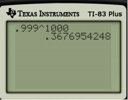

 ? Then the probability would be
  .
.
 , so that the probability of never winning for both problems is approximately
  .
.
 , we find
 , we have
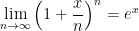
![\ln \left[ \displaystyle \lim_{n \to \infty} \left(1 + \frac{x}{n}\right)^n \right] = \displaystyle \lim_{n \to \infty} \ln \left[ \left(1 + \frac{x}{n}\right)^n \right]](https://s0.wp.com/latex.php?latex=%5Cln+%5Cleft%5B+%5Cdisplaystyle+%5Clim_%7Bn+%5Cto+%5Cinfty%7D+%5Cleft%281+%2B+%5Cfrac%7Bx%7D%7Bn%7D%5Cright%29%5En+%5Cright%5D+%3D+%5Cdisplaystyle+%5Clim_%7Bn+%5Cto+%5Cinfty%7D+%5Cln+%5Cleft%5B+%5Cleft%281+%2B+%5Cfrac%7Bx%7D%7Bn%7D%5Cright%29%5En+%5Cright%5D&bg=ffffff&fg=000000&s=0&c=20201002)
![\ln \left[ \displaystyle \lim_{n \to \infty} \left(1 + \frac{x}{n}\right)^n \right] = \displaystyle \lim_{n \to \infty} n \ln \left(1 + \frac{x}{n}\right)](https://s0.wp.com/latex.php?latex=%5Cln+%5Cleft%5B+%5Cdisplaystyle+%5Clim_%7Bn+%5Cto+%5Cinfty%7D+%5Cleft%281+%2B+%5Cfrac%7Bx%7D%7Bn%7D%5Cright%29%5En+%5Cright%5D+%3D+%5Cdisplaystyle+%5Clim_%7Bn+%5Cto+%5Cinfty%7D+n+%5Cln+%5Cleft%281+%2B+%5Cfrac%7Bx%7D%7Bn%7D%5Cright%29&bg=ffffff&fg=000000&s=0&c=20201002)
![\ln \left[ \displaystyle \lim_{n \to \infty} \left(1 + \frac{x}{n}\right)^n \right] = \displaystyle \lim_{n \to \infty} \frac{ \displaystyle \ln \left(1 + \frac{x}{n}\right)}{\displaystyle \frac{1}{n}}](https://s0.wp.com/latex.php?latex=%5Cln+%5Cleft%5B+%5Cdisplaystyle+%5Clim_%7Bn+%5Cto+%5Cinfty%7D+%5Cleft%281+%2B+%5Cfrac%7Bx%7D%7Bn%7D%5Cright%29%5En+%5Cright%5D+%3D+%5Cdisplaystyle+%5Clim_%7Bn+%5Cto+%5Cinfty%7D+%5Cfrac%7B+%5Cdisplaystyle+%5Cln+%5Cleft%281+%2B+%5Cfrac%7Bx%7D%7Bn%7D%5Cright%29%7D%7B%5Cdisplaystyle+%5Cfrac%7B1%7D%7Bn%7D%7D&bg=ffffff&fg=000000&s=0&c=20201002)
 as
as  , and so we may use L’Hopital’s rule, differentiating both the numerator and the denominator with respect to
  .
.![\ln \left[ \displaystyle \lim_{n \to \infty} \left(1 + \frac{x}{n}\right)^n \right] = \displaystyle \lim_{n \to \infty} \frac{ \displaystyle \frac{1}{1 + \frac{x}{n}} \cdot \frac{-x}{n^2} }{\displaystyle \frac{-1}{n^2}}](https://s0.wp.com/latex.php?latex=%5Cln+%5Cleft%5B+%5Cdisplaystyle+%5Clim_%7Bn+%5Cto+%5Cinfty%7D+%5Cleft%281+%2B+%5Cfrac%7Bx%7D%7Bn%7D%5Cright%29%5En+%5Cright%5D+%3D+%5Cdisplaystyle+%5Clim_%7Bn+%5Cto+%5Cinfty%7D+%5Cfrac%7B+%5Cdisplaystyle+%5Cfrac%7B1%7D%7B1+%2B+%5Cfrac%7Bx%7D%7Bn%7D%7D+%5Ccdot+%5Cfrac%7B-x%7D%7Bn%5E2%7D+%7D%7B%5Cdisplaystyle+%5Cfrac%7B-1%7D%7Bn%5E2%7D%7D&bg=ffffff&fg=000000&s=0&c=20201002)
![\ln \left[ \displaystyle \lim_{n \to \infty} \left(1 + \frac{x}{n}\right)^n \right] = \displaystyle \lim_{n \to \infty} \displaystyle \frac{x}{1 + \frac{x}{n}}](https://s0.wp.com/latex.php?latex=%5Cln+%5Cleft%5B+%5Cdisplaystyle+%5Clim_%7Bn+%5Cto+%5Cinfty%7D+%5Cleft%281+%2B+%5Cfrac%7Bx%7D%7Bn%7D%5Cright%29%5En+%5Cright%5D+%3D+%5Cdisplaystyle+%5Clim_%7Bn+%5Cto+%5Cinfty%7D+%5Cdisplaystyle+%5Cfrac%7Bx%7D%7B1+%2B+%5Cfrac%7Bx%7D%7Bn%7D%7D&bg=ffffff&fg=000000&s=0&c=20201002)
![\ln \left[ \displaystyle \lim_{n \to \infty} \left(1 + \frac{x}{n}\right)^n \right] = \displaystyle \frac{x}{1 + 0}](https://s0.wp.com/latex.php?latex=%5Cln+%5Cleft%5B+%5Cdisplaystyle+%5Clim_%7Bn+%5Cto+%5Cinfty%7D+%5Cleft%281+%2B+%5Cfrac%7Bx%7D%7Bn%7D%5Cright%29%5En+%5Cright%5D+%3D+%5Cdisplaystyle+%5Cfrac%7Bx%7D%7B1+%2B+0%7D&bg=ffffff&fg=000000&s=0&c=20201002)
![\ln \left[ \displaystyle \lim_{n \to \infty} \left(1 + \frac{x}{n}\right)^n \right] = x](https://s0.wp.com/latex.php?latex=%5Cln+%5Cleft%5B+%5Cdisplaystyle+%5Clim_%7Bn+%5Cto+%5Cinfty%7D+%5Cleft%281+%2B+%5Cfrac%7Bx%7D%7Bn%7D%5Cright%29%5En+%5Cright%5D+%3D+x&bg=ffffff&fg=000000&s=0&c=20201002)

 can be derived from the formula for discrete compound interest
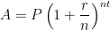


 and work backwards. This isn’t the best of logic — since we’re assuming the thing that we’re trying to prove in the first place — but it’s a helpful exercise to see exactly how this happened.


 . So, running the logic from bottom to top (and keeping in mind that all of the terms are positive), we obtain the top equation.
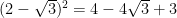


 ,
,  , and
, and  . The traditional method for finding the area of this circle would be to use the distance formula to find the length of each side and the height before plugging and chugging with the formula
  . Matrices can be used to compute the same area in fewer steps using the fact that the area of a triangle the absolute value of one-half times the determinant of a matrix containing the vertices of the triangle as shown below.
 , making the area positive eight instead of negative eight.


 .
.


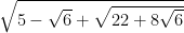
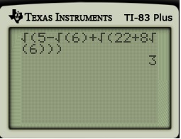
 and
and  . The challenge: fill in the rest without a calculator.
 , and
, and  — can be found exactly since they’re powers of
  ,
,  , and
, and 

 .
. .
. .
. .
. , or
, or  . So
. So
 into something more tangible and comfortable, like positive integers.
 for
for  and
and  for
for  .
. ,
,  is not much larger than
  . This is another way of saying that the graph of
  increases very slowly as
  are used to construct the unevenly-spaced lines and/or tick marks in