Mathematical induction and blank space

I tried out a one-liner in class that I’d been itching to try all summer.

I was introducing my students to proofs by mathematical induction; my example was showing that

$1 + 3 + 5 + \dots + (2n-1) = n^2$ .

After describing the principle of mathematical induction, I wrote out the $n = 1$ step and the assumption for $n = k$ :

$n=1$ : $1=1^2$ , so this checks.

$n =k$ : Assume that $1 + 3 + 5 + \dots + (2k-1) = k^2$ .

Then, for the inductive step, I had my students tell me what the left- and right-hand side would be if I substituted $k+1$ in place of $n$ . I wrote the answer for the left-hand side at the top of the board, the answer for the right-hand side at the bottom of the board, and left plenty of blank space in between the two (which I would fill in shortly):

$n = k+1$ :

$1 + 3 + 5 \dots + (2k-1) + (2[k+1]-1) =$

$~$

$= (k+1)^2$

So I explained that, to complete the proof by induction, all we had to do was convert the top line into the bottom line.

As my class swallowed hard as they thought about how to perform this task, I told them, “Yes, this looks really intimidating. Indeed, to quote the great philosopher, ‘You might think that I’m insane. But I’ve got a blank space, baby… and I’ll write your name.’ “

The one-liner provoked the desired response from my students… and after the laughter died down, we then worked through the end of the proof.

And, just in case you’ve been buried under a rock for the past few months, here’s the source material for the one-liner (which, at the time of this writing, is the second-most watched video on YouTube):

How Pixar uses math to make characters look perfect

Courtesy Gizmodo: http://gizmodo.com/how-pixar-uses-math-to-make-characters-look-perfect-1657339566

Simpson’s Rule and Sums of Powers

Source: https://www.facebook.com/AmerMathMonthly/photos/a.250425975006394.53155.241224542593204/737391462976507/?type=1&theater

Engaging students: Graphs of linear equations

In my capstone class for future secondary math teachers, I ask my students to come up with ideas for engaging their students with different topics in the secondary mathematics curriculum. In other words, the point of the assignment was not to devise a full-blown lesson plan on this topic. Instead, I asked my students to think about three different ways of getting their students interested in the topic in the first place.

I plan to share some of the best of these ideas on this blog (after asking my students’ permission, of course).

This student submission again comes from my former student Nada Al-Ghussain. Her topic, from Algebra: graphs of linear equations.

How could you as a teacher create an activity or project that involves your topic?

Positive slope, negative slope, no slope, and undefined, are four lines that cross over the coordinate plane. Boring. So how can I engage my students during the topic of graphs of linear equations, when all they can think of is the four images of slope? Simple, I assign a project that brings out the Individuality and creativity of each student. Something to wake up their minds!

An individualized image-graphing project. I would give each student a large coordinate plane, where they will graph their picture using straight lines only. I would ask them to use only points at intersections, but this can change to half points if needed. Then each student will receive an Equation sheet where they will find and write 2 equations for each different type of slope. So a student will have equations for two horizontal lines, vertical lines, positive slope, and negative slope. The best part is the project can be tailored to each class weakness or strength. I can also ask them to write the slop-intercept form, point slope form, or to even compare slopes that are parallel or perpendicular. When they are done, students would have practiced graphing and writing linear equations many times using their drawn images. Some students would be able to recognize slopes easier when they recall this project and their specific work on it.

Example of a project template:

Examples of student work:

How has this topic appeared in the news?

Millions of people tune in to watch the news daily. Information is poured into our ears and images through our eyes. We cannot absorb it all, so the news makes it easy for us to understand and uses graphs of linear equations. Plus, the Whoa! Factor of the slopping lines is really the attention grabber. News comes in many forms either through, TV, Internet, or newspaper. Students can learn to quickly understand the meaning of graphs with the different slopes the few seconds they are exposed to them.

On television, FOX news shows a positive slope of increasing number of job losses through a few years. (Beware for misrepresented data!)

A journal article contains the cost of college increase between public and private colleges showing the negative slope of private costs decreasing.

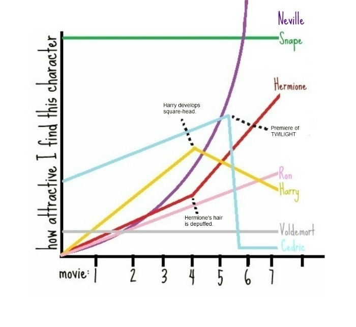
Most importantly line graphs can help muggles, half bloods, witches, and wizards to better understand the rise and decline of attractive characters through the Harry Potter series.

How can this topic be used in your students’ future courses in mathematics or science?

Students are introduced to simple graphs of linear equations where they should be able to name and find the equation of the slope. In a student’s future course with computers or tablets, I would use the Desmos graphing calculator online. This tool gives the students the ability to work backwards. I would ask a class to make certain lines, and they will have to come up with the equation with only their knowledge from previous class. It would really help the students understand the reason behind a negative slope and positive slope plus the difference between zero slope and undefined. After checking their previous knowledge, students can make visual representations of graphing linear inequalities and apply them to real-world problems.

References:

http://www.hoppeninjamath.com/teacherblog/?p=217

http://walkinginmathland.weebly.com/teaching-math-blog/animal-project-graphing-linear-lines-and-stating-equations

http://mediamatters.org/research/2012/10/01/a-history-of-dishonest-fox-charts/190225

http://money.cnn.com/2010/10/28/pf/college/college_tuition/

http://dailyfig.figment.com/2011/07/13/harry-potter-in-charts/

https://www.desmos.com/calculator

Multiplication and Animaniacs

One of my guilty pleasures in the 1990s, when I was far too old to be watching children’s cartoons, was the fantastic show “Animaniacs.” In the clip below, Yakko Warner describes how to multiply 47 and 83.

Preparation for Industrial Careers in the Mathematical Sciences: Improving Market Strategies

The Mathematical Association of America recently published a number of promotional videos showing various mathematics can be used in “the real world.” Here’s the fourth pair of videos describing how mathematics is used in the world of finance. From the YouTube descriptions:

Dr. Jonathan Adler (winner of King of the Nerds Season 3) talks about his career path and about a specific research problem that he has worked on. Using text analytics he was able to help an online company distinguish between its business customers and its private consumers from gift card messages.

Prof. Talithia Williams of Harvey Mudd College explains the statistical techniques that can be used to classify customers of a company using the messages on their gift cards.

How I Impressed My Wife: Part 7

And so I’ve finally arrived at the end of this series, describing what one of my professors called the art of integration. I really liked that phrase, and I’ve passed that on to my own students.

I really like the integral

$\displaystyle \int_0^{2\pi} \frac{dx}{\cos^2 x + 2 a \sin x \cos x + (a^2 + b^2) \sin^2 x}$

because there are so many different ways of evaluating it, as discussed in this series. Indeed, when I started typing out this series, I never imagined that I had enough material to fill a series with more than 40 entries! These techniques include:

Ordinary substitutions
Trigonometric substitutions
Trigonometric identities… lots of trigonometric identities
The magic substitution $u = \tan x/2$
Completing the square
Eliminating unneeded parameters
Differentiation under the integral sign (see Wikipedia for more details about this most untaught way of computing integrals)
Partial fractions… and different ways of obtaining a partial fractions decomposition
The substitution $z = e^{i x}$ , converting an integral on $[0,2\pi]$ to a contour integral over the unit circle in the complex plane.
Converting an integral on $(-\infty,\infty)$ to the limit of a contour integral over a semicircle in the complex plane.
Residues… and different ways of computing the residue at a pole

I don’t claim to have exhausted all of the ways that this integral can be computed; please leave a comment if you think you’ve found a technique that is substantially different than those I’ve already presented.

Back when I was a student, my calculus professor said that differentiation was a science. There are rules to follow (the Chain Rule, the Product Rule, the Quotient Rule, etc.), but that any function can be differentiated through the careful application of these rules. Integration, on the other hand, is more of an art. Yes, there are some techniques that need to be known, but often great creativity is needed in order to compute an integral. Differentiation does not require much creativity, but integration does. I thought that this was a profound insight for students just learning calculus, and so I’ve been passing this insight to my own students.

There are a couple loose threads in this series that I’d like to resolve one of these days:

I’d love to figure out a better way of showing that the above integral does not depend on $a$ without doing so much work toward computing it explicitly.
I’d love to figure out a way of computing the integral that results after the magic substitution is performed. The denominator becomes a messy quartic polynomial, and I haven’t figured out a good way of determining the roots of this polynomial. (I avoided this complication in this series by setting $a = 0$ , which did not ultimately affect the value of the integral.)

At the start of this series, I mentioned that this integral was original posed to me by my wife, who was trying to resolve a difference in the way that Mathematica 4 and Mathematica 8 computed it. In conclusion, I end with the Newton’s Three Laws story which was publicized in the following article that UNT publicized about my wife and me for Valentine’s Day 2015.

How I Impressed My Wife: Part 6g

This series was inspired by a question that my wife asked me: calculate

$Q = \displaystyle \int_0^{2\pi} \frac{dx}{\cos^2 x + 2 a \sin x \cos x + (a^2 + b^2) \sin^2 x}$

Originally, I multiplied the top and bottom of the integrand by $\tan^2 x$ and performed a substitution. However, as I’ve discussed in this series, there are four different ways that this integral can be evaluated.

Starting with today’s post, I’ll begin a fifth method. I really like this integral, as it illustrates so many different techniques of integration as well as the trigonometric tricks necessary for computing some integrals.

Since $Q$ is independent of $a$ , I can substitute any convenient value of $a$ that I want without changing the value of $Q$ . As shown in previous posts, substituting $a =0$ yields the following simplification:

$Q = \displaystyle \int_0^{2\pi} \frac{dx}{\cos^2 x + 2 a \sin x \cos x + (a^2 + b^2) \sin^2 x}$

$= \displaystyle \int_{0}^{2\pi} \frac{dx}{\cos^2 x + 2 \cdot 0 \cdot \sin x \cos x + (0^2 + b^2) \sin^2 x}$

$= \displaystyle \int_{0}^{2\pi} \frac{dx}{\cos^2 x + b^2 \sin^2 x}$

$= \displaystyle \int_{-\pi}^{\pi} \frac{dx}{\cos^2 x + b^2 \sin^2 x}$

$= \displaystyle \int_{-\infty}^{\infty} \frac{ 2(1+u^2) du}{u^4 + (4 b^2 - 2) u^2 + 1}$

$= \displaystyle \lim_{R \to \infty} \oint_{C_R} \frac{ 2(1+z^2) dz}{z^4 + (4 b^2 - 2) z^2 + 1}$

$= 2\pi i \left[\displaystyle \frac{r_1}{r_1^2-1} + \displaystyle \frac{r_2}{r_2^2-1} \right]$ ,

where I’ve made the assumption that $|b| < 1$ . In the above derivation, $C_R$ is the contour in the complex plane shown below (graphic courtesy of Mathworld).

Also,

$r_1 = \sqrt{1-b^2} + |b|i$

and

$r_2 = -\sqrt{1-b^2} + |b|i$

are the two poles of the final integrand that lie within this contour.

It now remains to simplify the final algebraic expression. To begin, I note

$\displaystyle \frac{r_1}{r_1^2-1} = \displaystyle \frac{\sqrt{1-b^2} + |b|i}{[\sqrt{1-b^2} + |b|i]^2 - 1}$

$= \displaystyle \frac{\sqrt{1-b^2} + |b|i}{1-b^2 + 2|b|i\sqrt{1-b^2} - |b|^2 - 1}$

$= \displaystyle \frac{\sqrt{1-b^2} + |b|i}{-2|b|^2 + 2|b|i\sqrt{1-b^2}}$

$= \displaystyle \frac{\sqrt{1-b^2} + |b|i}{2|b|i(|b|i +\sqrt{1-b^2})}$

$= \displaystyle \frac{1}{2|b|i}$ .

Similarly,

$\displaystyle \frac{r_2}{r_2^2-1} = \displaystyle \frac{-\sqrt{1-b^2} + |b|i}{[-\sqrt{1-b^2} + |b|i]^2 - 1}$

$= \displaystyle \frac{-\sqrt{1-b^2} + |b|i}{1-b^2 - 2|b|i\sqrt{1-b^2} - |b|^2 - 1}$

$= \displaystyle \frac{-\sqrt{1-b^2} + |b|i}{-2|b|^2 - 2|b|i\sqrt{1-b^2}}$

$= \displaystyle \frac{-\sqrt{1-b^2} + |b|i}{2|b|i(|b|i -\sqrt{1-b^2})}$

$= \displaystyle \frac{1}{2|b|i}$ .

Therefore,

$Q = 2\pi i \left[\displaystyle \frac{r_1}{r_1^2-1} + \displaystyle \frac{r_2}{r_2^2-1} \right] = 2\pi i \left[ \displaystyle \frac{1}{2|b|i} + \frac{1}{2|b| i} \right] = 2\pi i \displaystyle \frac{2}{2|b|i} = \displaystyle \frac{2\pi}{|b|}$ .

And so, at long last, I’ve completed a fifth different evaluation of $Q$ .

How I Impressed My Wife: Part 6f

This series was inspired by a question that my wife asked me: calculate

$Q = \displaystyle \int_0^{2\pi} \frac{dx}{\cos^2 x + 2 a \sin x \cos x + (a^2 + b^2) \sin^2 x}$

$= \displaystyle \int_{0}^{2\pi} \frac{dx}{\cos^2 x + 2 \cdot 0 \cdot \sin x \cos x + (0^2 + b^2) \sin^2 x}$

$= \displaystyle \int_{0}^{2\pi} \frac{dx}{\cos^2 x + b^2 \sin^2 x}$

$= \displaystyle \int_{-\pi}^{\pi} \frac{dx}{\cos^2 x + b^2 \sin^2 x}$

$= \displaystyle \int_{-\infty}^{\infty} \frac{ 2(1+u^2) du}{u^4 + (4 b^2 - 2) u^2 + 1}$

$= \displaystyle \lim_{R \to \infty} \oint_{C_R} \frac{ 2(1+z^2) dz}{z^4 + (4 b^2 - 2) z^2 + 1}$ ,

where $C_R$ is the contour in the complex plane shown below (graphic courtesy of Mathworld).

Amazingly, contour integrals can be simply computed by evaluating the residues at every pole located inside of the contour. (See Wikipedia and Mathworld for more details.) I have already handled the case of $|b| = 1$ and $|b| > 1$ . Today, I begin the final case of $|b| < 1$ .

Earlier in this series, I showed that

$z^4 + (4b^2 - 2) z^2 + 1 = (z^2 + 2z \sqrt{1-b^2} + 1)(z^2 - 2z \sqrt{1-b^2} + 1)$

if $|b| < 1$ , and so the quadratic formula can be used to find the four poles of the integrand:

$r_1 = \sqrt{1-b^2} + |b|i$ ,

$r_2 = -\sqrt{1-b^2} + |b|i$ ,

$r_3 = \sqrt{1-b^2} - |b|i$ ,

$r_4 = -\sqrt{1-b^2} - |b|i$ .

Of these, only two lie ( $r_1$ and $r_2$ ) within the contour for sufficiently large $R$ (actually, for $R > 1$ since all four poles lie on the unit circle in the complex plane).

As shown earlier in this series, the residue at each pole is given by

$\displaystyle \frac{r^2 + 1}{2r^3 + (4b^2-2)r}$

I’ll now simplify this considerably by using the fact that $r^4 + (4b^2-2)r^2 + 1 = 0$ at each pole:

$\displaystyle \frac{r^2 + 1}{2r^3 + (4b^2-2)r} = \displaystyle \frac{r(r^2+1)}{2r^4+(4b^2)-r^2}$

$= \displaystyle \frac{r(r^2+1)}{r^4+r^4 + (4b^2)-r^2}$

$= \displaystyle \frac{r(r^2+1)}{r^4-1}$

$= \displaystyle \frac{r(r^2+1)}{(r^2+1)(r^2-1)}$

$= \displaystyle \frac{r}{r^2-1}$ .

Therefore, to evaluate the contour integral, I simply the sum of the residues within the contour and multiply the sum by $2\pi i$ :

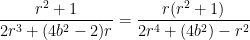
$Q = \displaystyle \lim_{R \to \infty} \oint_{C_R} \frac{ 2(1+z^2) dz}{z^4 + (4 b^2 - 2) z^2 + 1} = 2\pi i \left[\displaystyle \frac{r_1}{r_1^2-1} + \displaystyle \frac{r_2}{r_2^2-1} \right]$ .

So, to complete the evaluation of $Q$ , I need to simplify the right-hand side. I’ll complete this in tomorrow’s post.

How I Impressed My Wife: Part 6e

This series was inspired by a question that my wife asked me: calculate

$Q = \displaystyle \int_0^{2\pi} \frac{dx}{\cos^2 x + 2 a \sin x \cos x + (a^2 + b^2) \sin^2 x}$

nvenient value of $a$ that I want without changing the value of $Q$ . As shown in previous posts, substituting $a =0$ yields the following simplification:

$Q = \displaystyle \int_0^{2\pi} \frac{dx}{\cos^2 x + 2 a \sin x \cos x + (a^2 + b^2) \sin^2 x}$

$= \displaystyle \int_{0}^{2\pi} \frac{dx}{\cos^2 x + 2 \cdot 0 \cdot \sin x \cos x + (0^2 + b^2) \sin^2 x}$

$= \displaystyle \int_{0}^{2\pi} \frac{dx}{\cos^2 x + b^2 \sin^2 x}$

$= \displaystyle \int_{-\pi}^{\pi} \frac{dx}{\cos^2 x + b^2 \sin^2 x}$

$= \displaystyle \int_{-\infty}^{\infty} \frac{ 2(1+u^2) du}{u^4 + (4 b^2 - 2) u^2 + 1}$

$= \displaystyle \lim_{R \to \infty} \oint_{C_R} \frac{ 2(1+z^2) dz}{z^4 + (4 b^2 - 2) z^2 + 1}$

$= 2\pi \displaystyle \left[ \frac{1-r_1^2}{-2r_1^3 + (4b^2-2) r_1} +\frac{1-r_2^2}{-2r_2^3 + (4b^2-2) r_2} \right]$

where I’ve assumed $|b| > 1$ , the contour $C_R$ in the complex plane is shown below (graphic courtesy of Mathworld),

and the positive constants $r_1$ and $r_2$ are given by

$r_1 = \sqrt{2b^2 - 1 + 2|b| \sqrt{b^2 - 1}}$ ,

$r_2 = \sqrt{2b^2 - 1 - 2|b| \sqrt{b^2 - 1}}$ .

Now we have the small matter of simplifying our expression for $Q$ . Actually, this isn’t a small matter because Mathematica 10.1 is not able to simplify this expression much at all:

Fortunately, humans can still do some things that computers can’t. The numbers $r_1$ and $r_2$ are chosen so that $\pm ir_1$ and $\pm ir_2$ are the roots of the denominator $z^4 + (4 b^2 - 2) z^2 + 1$ . In other words,

$[ir_1]^4 + (4b^2 - 2) [ir_1]^2 + 1 = r_1^4 - [4b^2-2] r_1^2 + 1 = 0$ ,

$r_2^4 - [4b^2-2] r_2^2 + 1 = 0$

These relationships will be very handy for simplifying our expression for $Q$ :

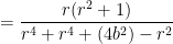
$Q = 2\pi \displaystyle \left[ \frac{1-r_1^2}{-2r_1^3 + (4b^2-2) r_1} +\frac{1-r_2^2}{-2r_2^3 + (4b^2-2) r_2} \right]$

$= 2\pi \left[ \displaystyle \frac{r_1^2-1}{2r_1^3-(4b^2-2)r_1} + \frac{r_2^2-1}{2r_2^3-(4b^2-2)r_2} \right]$

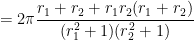
$= 2\pi \left[ \displaystyle \frac{r_1(r_1^2-1)}{2r_1^4-(4b^2-2)r_1^2} + \frac{r_2(r_2^2-1)}{2r_2^4-(4b^2-2)r_2^2} \right]$

$= 2\pi \left[ \displaystyle \frac{r_1(r_1^2-1)}{r_1^4 + r_1^4-(4b^2-2)r_1^2} + \frac{r_2(r_2^2-1)}{r_2^4+r_2^4-(4b^2-2)r_2^2} \right]$

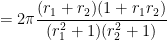
$= 2\pi \left[ \displaystyle \frac{r_1(r_1^2-1)}{r_1^4 -1} + \frac{r_2(r_2^2-1)}{r_2^4-1} \right]$

$= 2\pi \left[ \displaystyle \frac{r_1(r_1^2-1)}{(r_1^2 -1)(r_1^2+1)} + \frac{r_2(r_2^2-1)}{(r_2^2-1)(r_2^2+1)} \right]$

$= 2\pi \left[ \displaystyle \frac{r_1}{r_1^2+1} + \frac{r_2}{r_2^2+1} \right]$

$= 2\pi \displaystyle \frac{r_1(r_2^2+1)+(r_1^2+1)r_2}{(r_1^2+1)(r_2^2+1)}$

$= 2\pi \displaystyle \frac{r_1 r_2^2+r_1+r_1^2 r_2 +r_2}{(r_1^2+1)(r_2^2+1)}$

$= 2\pi \displaystyle \frac{r_1 +r_2 + r_1 r_2 (r_1 + r_2)}{(r_1^2+1)(r_2^2+1)}$

$= 2\pi \displaystyle \frac{(r_1 +r_2)(1 + r_1 r_2)}{(r_1^2+1)(r_2^2+1)}$

To complete the calculation, we recall that

$r_1 = \sqrt{2b^2 - 1 + 2|b| \sqrt{b^2 - 1}}$ ,

$r_2 = \sqrt{2b^2 - 1 - 2|b| \sqrt{b^2 - 1}}$ ,

so that

$r_1^2 + r_2^2 = 4b^2 - 2$ ,

$r_1^2 r_2^2 = 1$ ,

and hence

$r_1 r_2 = 1$

since $r_1$ and $r_2$ are both positive. Also,

$(r_1 + r_2)^2 = r_1^2 + 2r_1 r_2 + r_2^2 = 4b^2 -2 + 2 = 4b^2$ ,

so that

$r_1 + r_2 = 2|b|$ .

Finally,

$(r_1^2 + 1)(r_2^2 + 1) = (2b^2 + 2|b| \sqrt{b^2-1})(2b^2 - 2|b| \sqrt{b^2 -1})$

$= 4b^4 - 4b^2 (b^2-1)$

$= 4b^2$ .

Therefore,

$Q = 2\pi \displaystyle \frac{(r_1 +r_2)(1 + r_1 r_2)}{(r_1^2+1)(r_2^2+1)} = 2\pi \displaystyle \frac{ 2|b| \cdot (1 + 1)}{4b^2} = \displaystyle \frac{8\pi |b|}{4 |b|^2} = \displaystyle \frac{2\pi}{|b|}$ .

So far, I’ve evaluated the integral $Q$ for the cases $|b| = 1$ and $|b| > 1$ . Beginning with tomorrow’s post, I’ll evaluate the integral for the case $|b| < 1$ . As it turns out, the method presented above will again be utilized for simplifying the two residues.