In this series, I’m discussing how ideas from calculus and precalculus (with a touch of differential equations) can predict the precession in Mercury’s orbit and thus confirm Einstein’s theory of general relativity. The origins of this series came from a class project that I assigned to my Differential Equations students maybe 20 years ago.
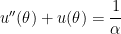
We previously showed that if the motion of a planet around the Sun is expressed in polar coordinates  , with the Sun at the origin, then under Newtonian mechanics (i.e., without general relativity) the motion of the planet follows the differential equation
 ,
,
where  and
and  is a certain constant. We will also impose the initial condition that the planet is at perihelion (i.e., is closest to the sun), at a distance of
  , when
  . This means that
  obtains its maximum value of
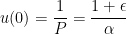
  when . This leads to the two initial conditions
 ;
;
the second equation arises since has a local extremum at .
In the previous post, we confirmed that

solved this initial-value problem. However, the solution was unsatisfying because it gave no indication of where this guess might have come from. In this post, I suggest a series of questions that good calculus students could be asked that would hopefully lead them quite naturally to this solution.
Step 1. Let’s make the differential equation simpler, for now, by replacing the right-hand side with 0:
 ,
,
or
 .
.
Can you think of a function or two that, when you differentiate twice, you get the original function back, except with a minus sign in front?
Answer to Step 1. With a little thought, hopefully students can come up with the standard answers of  and
and  .
.
Step 2. Using these two answers, can you think of a third function that works?
Answer to Step 2. This is usually the step that students struggle with the most, as they usually try to think of something completely different that works. This won’t work, but that’s OK… we all learn from our failures. If they can’t figure out, I’ll give a big hint: “Try multiplying one of these two answers by something.” In time, they’ll see that answers like  and
and  work. Once that conceptual barrier is broken, they’ll usually produce the solutions
  and
and  .
.
Step 3. Using these two answers, can you think of anything else that works?
Answer to Step 3. Again, students might struggle as they imagine something else that works. If this goes on for too long, I’ll give a big hint: “Try combining them.” Eventually, we hopefully get to the point that they’ll see that the linear combination  also solves the associated homogeneous differential equation.
Step 4. Let’s now switch back to the original differential equation . Let’s start simple:  . Can you think of an easy function that’s a solution?
Answer to Step 4. This might take some experimentation, and students will probably try unnecessarily complicated guesses first. If this goes on for too long, I’ll give a big hint: “Try a constant.” Eventually, they hopefully determine that if  is a constant function, then clearly
  and
and  , so that .
Step 5. Let’s return to . Any guesses on an answer to this one?
Answer to Step 5. Hopefully, students quickly realize that the constant function  works.
Step 6. Let’s review. We’ve shown that anything of the form  is a solution of . We’ve also shown that
  is a solution of . Can you think use these two answers to find something else that works?
Answer to Step 6. Hopefully, with the experience learned from Step 3, students will guess that  will work.
Step 7. OK, that solves the differential equation. Any thoughts on how to find the values of  and
and  so that
  and
and  ?
?
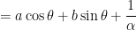
Answer to Step 7. Hopefully, students will see that we should just plug into  :
:



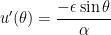
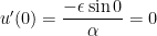
To find , we first find  and then substitute :


 .
.
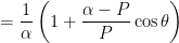
From these two constants, we obtain

 ,
,
where  .
.
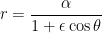
Finally, since  , we see that the planet’s orbit satisfies
 ,
,
so that, as shown earlier in this series, the orbit is an ellipse with eccentricity  .
.












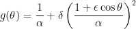

![f_1(\theta) = -\displaystyle \int \left[ \frac{1}{\alpha} + \delta \left( \frac{1 + \epsilon \cos \theta}{\alpha} \right)^2 \right] \sin \theta \, d\theta](https://s0.wp.com/latex.php?latex=f_1%28%5Ctheta%29+%3D+-%5Cdisplaystyle+%5Cint+%5Cleft%5B+%5Cfrac%7B1%7D%7B%5Calpha%7D+%2B+%5Cdelta+%5Cleft%28+%5Cfrac%7B1+%2B+%5Cepsilon+%5Ccos+%5Ctheta%7D%7B%5Calpha%7D+%5Cright%29%5E2+%5Cright%5D+%5Csin+%5Ctheta+%5C%2C+d%5Ctheta&bg=ffffff&fg=000000&s=0&c=20201002)
![= \displaystyle \int \left[ \frac{1}{\alpha} + \delta \left( \frac{1 + \epsilon t}{\alpha} \right)^2 \right] \, dt](https://s0.wp.com/latex.php?latex=%3D+%5Cdisplaystyle+%5Cint+%5Cleft%5B+%5Cfrac%7B1%7D%7B%5Calpha%7D+%2B+%5Cdelta+%5Cleft%28+%5Cfrac%7B1+%2B+%5Cepsilon+t%7D%7B%5Calpha%7D+%5Cright%29%5E2+%5Cright%5D+%5C%2C+dt&bg=ffffff&fg=000000&s=0&c=20201002)


![f_2(\theta) = \displaystyle \int \left[ \frac{1}{\alpha} + \delta \left( \frac{1 + \epsilon \cos \theta}{\alpha} \right)^2 \right] \cos\theta \, d\theta](https://s0.wp.com/latex.php?latex=f_2%28%5Ctheta%29+%3D+%5Cdisplaystyle+%5Cint+%5Cleft%5B+%5Cfrac%7B1%7D%7B%5Calpha%7D+%2B+%5Cdelta+%5Cleft%28+%5Cfrac%7B1+%2B+%5Cepsilon+%5Ccos+%5Ctheta%7D%7B%5Calpha%7D+%5Cright%29%5E2+%5Cright%5D+%5Ccos%5Ctheta+%5C%2C+d%5Ctheta&bg=ffffff&fg=000000&s=0&c=20201002)
![f_2(\theta) = \displaystyle \int \left[ \frac{\cos \theta}{\alpha} + \frac{\delta \cos \theta}{\alpha^2} + \frac{2 \delta \epsilon \cos^2 \theta}{\alpha^2} + \frac{\delta \epsilon^2 \cos^3 \theta}{\alpha^2} \right] \, d\theta](https://s0.wp.com/latex.php?latex=f_2%28%5Ctheta%29+%3D+%5Cdisplaystyle+%5Cint+%5Cleft%5B+%5Cfrac%7B%5Ccos+%5Ctheta%7D%7B%5Calpha%7D+%2B+%5Cfrac%7B%5Cdelta+%5Ccos+%5Ctheta%7D%7B%5Calpha%5E2%7D+%2B+%5Cfrac%7B2+%5Cdelta+%5Cepsilon+%5Ccos%5E2+%5Ctheta%7D%7B%5Calpha%5E2%7D+%2B+%5Cfrac%7B%5Cdelta+%5Cepsilon%5E2+%5Ccos%5E3+%5Ctheta%7D%7B%5Calpha%5E2%7D+%5Cright%5D+%5C%2C+d%5Ctheta&bg=ffffff&fg=000000&s=0&c=20201002)
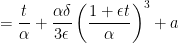
![= \displaystyle \int \left[ \frac{\cos \theta}{\alpha} + \frac{\delta \cos \theta}{\alpha^2} + \frac{\delta \epsilon (1 + \cos 2 \theta)}{\alpha^2} + \frac{\delta \epsilon^2 \cos \theta \cos^2 \theta}{\alpha^2} \right] \, d\theta](https://s0.wp.com/latex.php?latex=%3D+%5Cdisplaystyle+%5Cint+%5Cleft%5B+%5Cfrac%7B%5Ccos+%5Ctheta%7D%7B%5Calpha%7D+%2B+%5Cfrac%7B%5Cdelta+%5Ccos+%5Ctheta%7D%7B%5Calpha%5E2%7D+%2B+%5Cfrac%7B%5Cdelta+%5Cepsilon+%281+%2B+%5Ccos+2+%5Ctheta%29%7D%7B%5Calpha%5E2%7D+%2B+%5Cfrac%7B%5Cdelta+%5Cepsilon%5E2+%5Ccos+%5Ctheta+%5Ccos%5E2+%5Ctheta%7D%7B%5Calpha%5E2%7D+%5Cright%5D+%5C%2C+d%5Ctheta&bg=ffffff&fg=000000&s=0&c=20201002)
![= \displaystyle \int \left[ \frac{\cos \theta}{\alpha} + \frac{\delta \cos \theta}{\alpha^2} + \frac{\delta \epsilon}{\alpha^2} + \frac{\delta \epsilon \cos 2 \theta}{\alpha^2}+ \frac{\delta \epsilon^2 \cos \theta (1- \sin^2 \theta)}{\alpha^2} \right] \, d\theta](https://s0.wp.com/latex.php?latex=%3D+%5Cdisplaystyle+%5Cint+%5Cleft%5B+%5Cfrac%7B%5Ccos+%5Ctheta%7D%7B%5Calpha%7D+%2B+%5Cfrac%7B%5Cdelta+%5Ccos+%5Ctheta%7D%7B%5Calpha%5E2%7D+%2B+%5Cfrac%7B%5Cdelta+%5Cepsilon%7D%7B%5Calpha%5E2%7D+%2B+%5Cfrac%7B%5Cdelta+%5Cepsilon+%5Ccos+2+%5Ctheta%7D%7B%5Calpha%5E2%7D%2B+%5Cfrac%7B%5Cdelta+%5Cepsilon%5E2+%5Ccos+%5Ctheta+%281-+%5Csin%5E2+%5Ctheta%29%7D%7B%5Calpha%5E2%7D+%5Cright%5D+%5C%2C+d%5Ctheta&bg=ffffff&fg=000000&s=0&c=20201002)
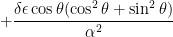
![= \displaystyle \int \left[ \frac{\cos \theta}{\alpha} + \frac{\delta (1 + \epsilon^2) \cos \theta}{\alpha^2} + \frac{\delta \epsilon}{\alpha^2} + \frac{\delta \epsilon \cos 2 \theta}{\alpha^2} - \frac{\delta \epsilon^2 \cos \theta \sin^2 \theta}{\alpha^2} \right] \, d\theta](https://s0.wp.com/latex.php?latex=%3D+%5Cdisplaystyle+%5Cint+%5Cleft%5B+%5Cfrac%7B%5Ccos+%5Ctheta%7D%7B%5Calpha%7D+%2B+%5Cfrac%7B%5Cdelta+%281+%2B+%5Cepsilon%5E2%29+%5Ccos+%5Ctheta%7D%7B%5Calpha%5E2%7D++%2B+%5Cfrac%7B%5Cdelta+%5Cepsilon%7D%7B%5Calpha%5E2%7D+%2B+%5Cfrac%7B%5Cdelta+%5Cepsilon+%5Ccos+2+%5Ctheta%7D%7B%5Calpha%5E2%7D+-+%5Cfrac%7B%5Cdelta+%5Cepsilon%5E2+%5Ccos+%5Ctheta+%5Csin%5E2+%5Ctheta%7D%7B%5Calpha%5E2%7D+%5Cright%5D+%5C%2C+d%5Ctheta&bg=ffffff&fg=000000&s=0&c=20201002)






















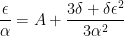
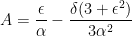




 .
.





 ,
, that was obtained earlier in this series.
 .
. .
. and
and 
 ,
,



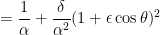
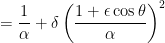 ,
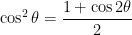
,
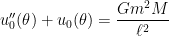 ,
, ,
,  .
.  ;
;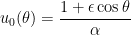 ,
, , we see that the planet’s orbit satisfies
![u''(\theta) + u(\theta) = \displaystyle \frac{Gm^2 M}{\ell^2} + \frac{3GM}{c^2} [u(\theta)]^2](https://s0.wp.com/latex.php?latex=u%27%27%28%5Ctheta%29+%2B+u%28%5Ctheta%29+%3D+%5Cdisplaystyle+%5Cfrac%7BGm%5E2+M%7D%7B%5Cell%5E2%7D+%2B+%5Cfrac%7B3GM%7D%7Bc%5E2%7D+%5Bu%28%5Ctheta%29%5D%5E2&bg=ffffff&fg=000000&s=0&c=20201002) ,
,![u''(\theta) + u(\theta) = \displaystyle \frac{1}{\alpha} + \delta [u(\theta)]^2](https://s0.wp.com/latex.php?latex=u%27%27%28%5Ctheta%29+%2B+u%28%5Ctheta%29+%3D+%5Cdisplaystyle+%5Cfrac%7B1%7D%7B%5Calpha%7D+%2B+%5Cdelta+%5Bu%28%5Ctheta%29%5D%5E2&bg=ffffff&fg=000000&s=0&c=20201002) ,
,![[u(\theta)]^2](https://s0.wp.com/latex.php?latex=%5Bu%28%5Ctheta%29%5D%5E2&bg=ffffff&fg=000000&s=0&c=20201002) .
. is very, very small, the solution of
 ![u''(\theta) + u(\theta) = \displaystyle \frac{1}{\alpha} + \delta [u_0(\theta)]^2](https://s0.wp.com/latex.php?latex=u%27%27%28%5Ctheta%29+%2B+u%28%5Ctheta%29+%3D+%5Cdisplaystyle+%5Cfrac%7B1%7D%7B%5Calpha%7D+%2B+%5Cdelta+%5Bu_0%28%5Ctheta%29%5D%5E2&bg=ffffff&fg=000000&s=0&c=20201002) ,
,
 , the integrals for
  ,
, ,
,

 .
. .
. is not a solution of the characteristic equation, this leads to trying something of the form
  as a solution, where
  is a standard technique from differential equations; later in this series, I’ll give some justification for this guess.)
 and
and  . Substituting, we find


 is a particular solution of the nonhomogeneous differential equation.
 .
. . Since
  is the reciprocal of
  is extremely unlikely, this means that the planet orbits the Sun in an ellipse, with the Sun at one focus of the ellipse.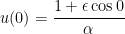


 .
. ,
, ,
,
 ,
, and the acceleration
  are vectors. When written in polar coordinates, this becomes
![{\bf F} = m \displaystyle \left[ \frac{d^2r}{dt^2} - r \left( \frac{d\theta}{dt} \right)^2 \right] {\bf u}_r + m \left(r \frac{d^2 \theta}{d t^2} + 2 \frac{dr}{dt} \frac{d\theta}{dt} \right) {\bf u}_\theta](https://s0.wp.com/latex.php?latex=%7B%5Cbf+F%7D+%3D+m+%5Cdisplaystyle+%5Cleft%5B+%5Cfrac%7Bd%5E2r%7D%7Bdt%5E2%7D+-+r+%5Cleft%28+%5Cfrac%7Bd%5Ctheta%7D%7Bdt%7D+%5Cright%29%5E2+%5Cright%5D+%7B%5Cbf+u%7D_r+%2B+m+%5Cleft%28r+%5Cfrac%7Bd%5E2+%5Ctheta%7D%7Bd+t%5E2%7D+%2B+2+%5Cfrac%7Bdr%7D%7Bdt%7D+%5Cfrac%7Bd%5Ctheta%7D%7Bdt%7D+%5Cright%29+%7B%5Cbf+u%7D_%5Ctheta&bg=ffffff&fg=000000&s=0&c=20201002) ,
, is a unit vector pointing away from the origin and
  is a unit vector perpendicular to
  .
. ,
,![m \displaystyle \left[ \frac{d^2r}{dt^2} - r \left( \frac{d\theta}{dt} \right)^2 \right] = \displaystyle -\frac{GMm}{r^2}](https://s0.wp.com/latex.php?latex=m+%5Cdisplaystyle+%5Cleft%5B+%5Cfrac%7Bd%5E2r%7D%7Bdt%5E2%7D+-+r+%5Cleft%28+%5Cfrac%7Bd%5Ctheta%7D%7Bdt%7D+%5Cright%29%5E2+%5Cright%5D+%3D+%5Cdisplaystyle+-%5Cfrac%7BGMm%7D%7Br%5E2%7D&bg=ffffff&fg=000000&s=0&c=20201002) ,
, .
. ,
,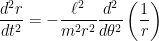 .
.


![\displaystyle \frac{\ell^2}{m^2 r^2} \left[ \frac{d^2}{d\theta^2} \left( \frac{1}{r} \right) + \frac{1}{r} \right] = \displaystyle \frac{GM}{r^2}](https://s0.wp.com/latex.php?latex=%5Cdisplaystyle++%5Cfrac%7B%5Cell%5E2%7D%7Bm%5E2+r%5E2%7D+%5Cleft%5B+%5Cfrac%7Bd%5E2%7D%7Bd%5Ctheta%5E2%7D+%5Cleft%28+%5Cfrac%7B1%7D%7Br%7D+%5Cright%29+%2B+%5Cfrac%7B1%7D%7Br%7D+%5Cright%5D++%3D+%5Cdisplaystyle+%5Cfrac%7BGM%7D%7Br%5E2%7D&bg=ffffff&fg=000000&s=0&c=20201002)
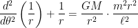
 .
. , we finally obtain the governing equation
 .
. as the constant on the right-hand side instead of just
