Confirming Einstein’s Theory of General Relativity With Calculus, Part 8: Second- and Third-Order Approximations

In this series, I’m discussing how ideas from calculus and precalculus (with a touch of differential equations) can predict the precession in Mercury’s orbit and thus confirm Einstein’s theory of general relativity. The origins of this series came from a class project that I assigned to my Differential Equations students maybe 20 years ago.

In this series, we found an approximate solution to the governing initial-value problem

$u''(\theta) + u(\theta) = \displaystyle \frac{1}{\alpha} + \delta [u(\theta)]^2$

$u(0) = \displaystyle \frac{1 + \epsilon}{\alpha}$

$u'(0) = 0$ ,

where $u = \displaystyle \frac{1}{r}$ , $\displaystyle \frac{1}{\alpha} = \frac{GMm^2}{\ell^2}$ , $\delta = \displaystyle \frac{3GM}{c^2}$ , $G$ is the gravitational constant of the universe, $m$ is the mass of the planet, $M$ is the mass of the Sun, $\ell$ is the constant angular momentum of the planet, $\epsilon$ is the eccentricity of the orbit, and $c$ is the speed of light.

We used the following steps to find an approximate solution.

Step 0. Ignore the general-relativity contribution and solve the simpler initial-value problem

$u_0''(\theta) + u_0(\theta) = \displaystyle \frac{1}{\alpha}$

$u_0(0) = \displaystyle \frac{1 + \epsilon}{\alpha}$

$u_0'(0) = 0$ ,

which is a zeroth-order approximation to the real initial-value problem. We found that the solution of this differential equation is

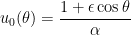
$u_0(\theta) = \displaystyle \frac{1 + \epsilon \cos \theta}{\alpha}$ ,

which is the equation of an ellipse in polar coordinates.

Step 1. Solve the initial-value problem

$u_1''(\theta) + u_1(\theta) = \displaystyle \frac{1}{\alpha} + \delta [u_0(\theta)]^2$

$u_1(0) = \displaystyle \frac{1 + \epsilon}{\alpha}$

$u_1'(0) = 0$ ,

which partially incorporates the term due to general relativity. This is a first-order approximation to the real differential equation. After much effort, we found that the solution of this initial-value problem is

$u_1(\theta) = \displaystyle \frac{1 + \epsilon \cos \theta}{\alpha} + \frac{\delta}{\alpha^2} + \frac{\delta \epsilon^2}{2\alpha^2} + \frac{ \delta\epsilon}{\alpha^2} \theta \sin \theta - \frac{ \delta \epsilon^2}{6\alpha^2} \cos 2\theta - \frac{\delta(3+\epsilon^2)}{3\alpha^2} \cos \theta$ .

For large values of $\theta$ , this is accurately approximated as:

$u_1(\theta) \approx \displaystyle \frac{1 + \epsilon \cos \theta}{\alpha} + \frac{ \delta\epsilon}{\alpha^2} \theta \sin \theta$ ,

which can be further approximated as

$u_1(\theta) \approx \displaystyle \frac{1}{\alpha} \left[ 1 + \epsilon \cos \left( \theta - \frac{\delta \theta}{\alpha} \right) \right]$ .

From this expression, the precession in a planet’s orbit due to general relativity can be calculated.

Roughly 20 years ago, I presented this application of differential equations at the annual meeting of the Texas Section of the Mathematical Association of America. After the talk, a member of the audience asked what would happen if we did this procedure yet again to find a second-order approximation. In other words, I was asked to consider…

Step 2. Solve the initial-value problem

$u_2''(\theta) + u_2(\theta) = \displaystyle \frac{1}{\alpha} + \delta [u_1(\theta)]^2$

$u_2(0) = \displaystyle \frac{1 + \epsilon}{\alpha}$

$u_2'(0) = 0$ .

It stands to reason that the answer should be an even more accurate approximation to the true solution $u(\theta)$ .

I didn’t have an immediate answer for this question, but I can answer it now. Letting Mathematica do the work, here’s the answer:

Yes, it’s a mess. The term in red is $u_0(\theta)$ , while the term in yellow is the next largest term in $u_1(\theta)$ . Both of these appear in the answer to $u_2(\theta)$ .

The term in green is the next largest term in $u_2(\theta)$ , with the highest power of $\theta$ in the numerator and the highest power of $\alpha$ in the denominator. In other words,

$u_2(\theta) \approx \displaystyle \frac{1 + \epsilon \cos \theta}{\alpha} + \frac{ \delta\epsilon}{\alpha^2} \theta \sin \theta -\frac{\delta^2 \epsilon}{2\alpha^3} \theta^2 \cos \theta$ .

How does this compare to our previous approximation of

$u(\theta) \approx \displaystyle \frac{1}{\alpha} \left[ 1 + \epsilon \cos \left( \theta - \frac{\delta \theta}{\alpha} \right) \right]$ ?

Well, to a second-order Taylor approximation, it’s the same! Let

$f(x) = \displaystyle \frac{1}{\alpha} \left[ 1 + \epsilon \cos \left( \theta - x \right) \right]$ .

Expanding about $x = 0$ and treated $\theta$ as a constant, we find

$f(x) \approx f(0) + f'(0) x + \displaystyle \frac{f''(0)}{2} x^2 = \displaystyle \frac{1}{\alpha} \left[ 1 + \epsilon \cos \left( \theta\right) \right] + \frac{\epsilon}{\alpha} x \sin \theta - \frac{\epsilon}{2\alpha} x^2 \cos \theta$ .

Substituting $x = \displaystyle \frac{\delta \theta}{\alpha}$ yields the above approximation for $u_2(\theta)$ .

Said another way, proceeding to a second-order approximation merely provides additional confirmation for the precession of a planet’s orbit.

Just for the fun of it, I also used Mathematica to find the solution of Step 3:

Step 2. Solve the initial-value problem

$u_3''(\theta) + u_3(\theta) = \displaystyle \frac{1}{\alpha} + \delta [u_2(\theta)]^2$

$u_3(0) = \displaystyle \frac{1 + \epsilon}{\alpha}$

$u_3'(0) = 0$ .

I won’t copy-and-paste the solution from Mathematica; unsurpisingly, it’s really long. I will say that, unsurprisingly, the leading terms are

$u_3(\theta) \approx \displaystyle \frac{1 + \epsilon \cos \theta}{\alpha} + \frac{ \delta\epsilon}{\alpha^2} \theta \sin \theta -\frac{\delta^2 \epsilon}{2 \alpha^3} \theta^2 \cos \theta -\frac{\delta^3 \epsilon}{6\alpha^4} \theta^3 \sin \theta$ .

I said “unsurprisingly” because this matches the third-order Taylor polynomial of our precession expression. I don’t have time to attempt it, but surely there’s a theorem to be proven here based on this computational evidence.

One thought on “Confirming Einstein’s Theory of General Relativity With Calculus, Part 8: Second- and Third-Order Approximations”

Pingback: Confirming Einstein’s General Theory of Relativity with Calculus: Index – Mean Green Math

Confirming Einstein’s Theory of General Relativity With Calculus, Part 8: Second- and Third-Order Approximations

Published by John Quintanilla

One thought on “Confirming Einstein’s Theory of General Relativity With Calculus, Part 8: Second- and Third-Order Approximations”

Leave a comment Cancel reply

Share this:

Related

Published by John Quintanilla

One thought on “Confirming Einstein’s Theory of General Relativity With Calculus, Part 8: Second- and Third-Order Approximations”

Leave a comment Cancel reply