I’m in the middle of a series of posts concerning the elementary operation of computing a square root. This is such an elementary operation because nearly every calculator has a 
Today’s topic is the use of log tables. I’m guessing that many readers have either forgotten how to use a log table or else were never even taught how to use them. After showing how log tables were used in the past, I’ll conclude with some thoughts about its effectiveness for teaching students logarithms for the first time.
This will be a fairly long post about log tables. In the next post, I’ll discuss how log tables can be used to compute square roots.
To begin, let’s again go back to a time before the advent of pocket calculators… say, 1912.
Before the advent of pocket calculators, most professional scientists and engineers had mathematical tables for keeping the values of logarithms, trigonometric functions, and the like. The following images come from one of my prized possessions: College Mathematics, by Kaj L. Nielsen (Barnes & Noble, New York, 1958). Some saint gave this book to me as a child in the late 1970s; trust me, it was well-worn by the time I actually got to college.
With the advent of cheap pocket calculators, mathematical tables are a relic of the past. The only place that any kind of mathematical table common appears in modern use are in statistics textbooks for providing areas and critical values of the normal distribution, the Student 
That said, mathematical tables are not a relic of the remote past. When I was learning logarithms and trigonometric functions at school in the early 1980s — one generation ago — I distinctly remember that my school textbook had these tables in the back of the book.
And it’s my firm opinion that, as an exercise in history, log tables can still be used today to deepen students’ facility with logarithms. In this post and Part 4 of this series, I discuss how the log table can be used to compute logarithms and (using the language of past generations) antilogarithms without a calculator. In Part 5, I’ll discuss my opinions about the pedagogical usefulness of log tables, even if logarithms can be computed more easily nowadays with scientific calculators. In Part 6, I’ll return to square roots — specifically, how log tables can be used to find square roots.


How to use the table, Part 1. How do you read this table? The left-most column shows the ones digit and the tenths digit, while the top row shows the hundredths digit. So, for example, the bottom row shows ten different base-10 logarithms:


So, rather than punching numbers into a calculator, the table was used to find these logarithms. You’ll notice that these values match, to four decimal places, the values found on a modern calculator.
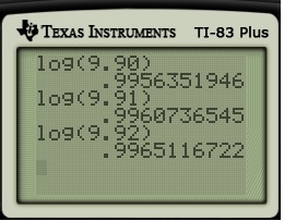
How to use the table, Part 2. What if we’re trying to take the logarithm of a number between 


So, to estimate 


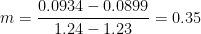
Finding this line is a straightforward exercise in the point-slope form of a line:


Remembering that this log table is only good to four significant digits, we estimate 
With a little practice, one can do the above calculations with relative ease. Also, many log tables of the past had a column called “proportional parts” that essentially replaced the step of linear interpolation, thus speeding the use of the table considerably.
Again, this matches the result of a modern calculator to four decimal places:

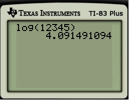
How to use the table, Part 3. So far, we’ve discussed taking the logarithms of numbers between 
To find 


More intuitively, we know that the answer must lie between 


We then find


Employing linear interpolation, we find


Remembering that this log table is only good to four significant digits, we estimate 

Again, this matches the result of a modern calculator to four decimal places (in this case, five significant digits):
How to use the table, Part 4. Let’s now consider what happens if we pick a positive number less than 


We have already found 


So that’s how to compute logarithms without a calculator: we rely on somebody else’s hard work to compute these logarithms (which were found in the back of every precalculus textbook a generation ago), and we make clever use of the laws of logarithms and linear interpolation.
Log tables are of course subject to roundoff errors. (For that matter, so are pocket calculators, but the roundoff happens so deep in the decimal expansion — the 12th or 13th digit — that students hardly ever notice the roundoff error and thus can develop the unfortunate habit of thinking that the result of a calculator is always exactly correct.)
For a two-page table found in a student’s textbook, the results were typically accurate to four significant digits. Professional engineers and scientists, however, needed more accuracy than that, and so they had entire books of tables. A table showing 5 places of accuracy would require about 20 printed pages, while a table showing 6 places of accuracy requires about 200 printed pages. Indeed, if you go to the old and dusty books of any decent university library, you should be able to find these old books of mathematical tables.
In other words, that’s how the Brooklyn Bridge got built in an era before pocket calculators.
At this point you may be asking, “OK, I don’t need to use a calculator to use a log table. But let’s back up a step. How were the values in the log table computed without a calculator?” That’s a perfectly reasonable question, but this post is getting long enough as it is. Perhaps I’ll address this issue in a future post.
 without a calculator? In the previous post, I introduced a trapping method that directly used the definition of
  , then the
  would have been in a group by itself.) I start with the
  . What perfect square is closest to
  . So, mimicking the algorithm for long division:
 s.
s. from
from 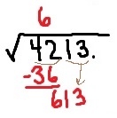
 .
. and under the
  –something times the same something to be as close to
  : too small
 : too small
 : too small
 : too small
 : too big
 on the next step.
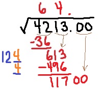
 .
. and under the
  –something times the same something to be as close to
  : too small
 : too small
 : too small
 : too small
 : too small
 : too small
 : too small
 : too small
 : still too small
 . We place the
  on the next step.
 .
. while waiting for the boarding announcement.
 somewhere (that was Step 1). So the basic problem is to solve for
  ,
, ,
, ,
,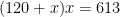
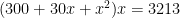
 , which was obtained at the start of Step 2. The left-hand side has the form
  as close to
  , we immediately see that
  , so that the answer lies between
  . To find the excess amount over 10, we need to solve
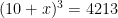 ,
, .
. as possible without going over.
 and see if we get it right.
 . Too small.
 . Too big.
 , the answer has to be somewhere between
  and
and  , let’s start by guessing
  .
. . Too big, but not much too big. So let’s try
  next, as opposed to
  or
or  .
. . Too small.
 , let’s start closer to


 and
and  or
or  .) Back in 1955, all of the above squaring was done by hand, without a calculator. With enough patience,


 is the amplitude of the tremor measured in micrometers and
  is the period of the tremor (time of one oscillation of the earth’s surface) measured in seconds.
 of a number
  defined as follows:
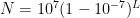
 .
.


 the base of the natural logarithm (which was also developed by Napier). While it is untrue, as is commonly believed, that Euler invented the number
  , he did give it the name
  . He was interested in the number because he wanted to calculate the amount that would result from continually compounded interested on a sum of money and the number
  and
and  . Of course, he knew that these rules were true and he could apply them in complex problems, but he didn’t know why they were true. And he wanted to have this deeper knowledge of mathematics beyond the ability to solve routine algebra problems.
 and
and  , this can be proven by repeated multiplication:
 repeated
  repeated
  times
times and
and  should be defined so that this rule still holds even if one (or both) of


 for positive integers


 .
.

 is negative, that
  . If it’s odd, multiply it by
  and then add
