Polynomial Long Division and Megan Moroney

A brief clip from Megan Moroney’s video “I’m Not Pretty” correctly uses polynomial long division to establish that $2x+3$ is a factor of $2x^4+5x^3+7x^2+16x+15$ . Even more amazingly, the fact that the remainder is $0$ actually fits artistically with the video.

And while I have her music on my mind, I can’t resist sharing her masterpiece “Tennessee Orange” and its playful commentary on the passion of college football fans.

Lagrange Points and Polynomial Equations: Index

I’m doing something that I should have done a long time ago: collecting a series of posts into one single post. The links below show my series on Lagrange points.

Part 1: Introduction

Part 2: Finding $L_1$

Part 3: Finding $L_2$

Part 4: A more analytical way of finding $L_1$ and $L_2$

Part 5: Historical anecdote: Lagrange made a careless mistake!

Solving Problems Submitted to MAA Journals (Part 3)

The following problem appeared in Volume 53, Issue 4 (2022) of The College Mathematics Journal.

Define, for every non-negative integer $n$ , the $n$ th Catalan number by

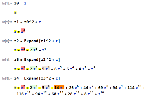
$C_n := \displaystyle \frac{1}{n+1} {2n \choose n}$ .

Consider the sequence of complex polynomials in $z$ defined by $z_k := z_{k-1}^2 + z$ for every non-negative integer $k$ , where $z_0 := z$ . It is clear that $z_k$ has degree $2^k$ and thus has the representation

$z_k =\displaystyle \sum_{n=1}^{2^k} M_{n,k} z^n$ ,

where each $M_{n,k}$ is a positive integer. Prove that $M_{n,k} = C_{n-1}$ for $1 \le n \le k+1$ .

This problem appeared in the same issue as the probability problem considered in the previous two posts. Looking back, I think that the confidence that I gained by solving that problem gave me the persistence to solve this problem as well.

My first thought when reading this problem was something like “This involves sums, polynomials, and binomial coefficients. And since the sequence is recursively defined, it’s probably going to involve a proof by mathematical induction. I can do this.”

My second thought was to use Mathematica to develop my own intuition and to confirm that the claimed pattern actually worked for the first few values of $z_k$ .

As claimed in the statement of the problem, each $z_k$ is a polynomial of degree $2^k$ without a nontrivial constant term. Also, for each $z_k$ , the term of degree $n$ , for $1 \le n \le k+1$ , has a coefficient that is independent of $k$ which equal to $C_{n-1}$ . For example, for $z_4$ , the coefficient of $z^5$ (in orange above) is equal to

$C_4 = \displaystyle \frac{1}{5} {8 \choose 4} = \frac{8!}{4! 4! \cdot 5} = \frac{40320}{2880} = 14$ ,

and the problem claims that the coefficient of $z^5$ will remain 14 for $z_5, z_6, z_7, \dots$

Confident that the pattern actually worked, all that remained was pushing through the proof by induction.

We proceed by induction on $k$ . The statement clearly holds for $k=1$ :

$z_1 = z_0^2 + z = z + z^2 = C_0 z + C_1 z^2$ .

Although not necessary, I’ll add for good measure that

$z_2 = z_1^2 + z = (z^2+z)^2 + z = z + z^2 + 2z^3 + z^4 = C_0 z + C_1 z^2 + C_2 z^3 + z^4$

and

$z_3 = z^2 + z = (z^4+2z^3+z^2+z)^2 + z$

$= z + z^2 + 2z^3 + 5z^4 + 6z^5 + 6z^6 + 4z^7 + z^8$

$= C_0 z + C_1 z^2 + C_2 z^3 + C_3 z^4 + 6z^5 + 6z^6 + 4z^7 + z^8.$

This next calculation illustrates what’s coming later. In the previous calculation, the coefficient of $z^4$ is found by multiplying out

$(z^4+2z^3+z^2+z)(z^4+2z^3+z^2+z)$ .

This is accomplished by examining all pairs, one from the left product and one from the right product, so that the exponent works out to be $z^4$ . In this case, it’s

$(2z^3)(z) + (z^2)(z^2) + (z)(2z^3) = 5z^4$ .

For the inductive step, we assume that, for some $k \ge 1$ , $M_{n,k} = C_{n-1}$ for all $1 \le n \le k+1$ , and we define

$z_{k+1} = z + \left( M_{1,k} z + M_{2,k} z^2 + M_{3,k} z^3 + \dots + M_{2^k,k} z^{2^k} \right)^2$

Our goal is to show that $M_{n,k+1} = C_{n-1}$ for $n = 1, 2, \dots, k+2$ .

For $n=1$ , the coefficient $M_{1,k+1}$ of $z$ in $z_{k+1}$ is clearly 1, or $C_0$ .

For $2 \le n \le k+2$ , the coefficient $M_{n,k+1}$ of $z^n$ in $z_{k+1}$ can be found by expanding the above square. Every product of the form $M_{j,k} z^j \cdot M_{n-j,k} z^{n-j}$ will contribute to the term $M_{n,k+1} z^n$ . Since $n \le k+2 \le 2^k+1$ (since $k \ge 1$ ), the values of $j$ that will contribute to this term will be $j = 1, 2, \dots, n-1$ . (Ordinarily, the $z^0$ and $z^n$ terms would also contribute; however, there is no $z^0$ term in the expression being squared). Therefore, after using the induction hypothesis and reindexing, we find

$M_{n,k+1} = \displaystyle \sum_{j=1}^{n-1} M_{j,k} M_{n-j,k}$

$= \displaystyle\sum_{j=1}^{n-1} C_{j-1} C_{n-j-1}$

$= \displaystyle\sum_{j=0}^{n-2} C_j C_{n-2-j}$

$= C_{n-1}$ .

The last step used a recursive relationship for the Catalan numbers that I vaguely recalled but absolutely had to look up to complete the proof.

Lagrange Points and Polynomial Equations: Part 4

From Wikipedia, Lagrange points are points of equilibrium for small-mass objects under the gravitational influence of two massive orbiting bodies. There are five such points in the Sun-Earth system, called $L_1$ , $L_2$ , $L_3$ , $L_4$ , and $L_5$ .

The stable equilibrium points $L_4$ and $L_5$ are easiest to explain: they are the corners of equilateral triangles in the plane of Earth’s orbit. The points $L_1$ and $L_2$ are also equilibrium points, but they are unstable. Nevertheless, they have practical applications for spaceflight.

As we’ve seen, the positions of $L_1$ and $L_2$ can be found by numerically solving the fifth-order polynomial equations

$t^5 - (3-\mu) t^4 + (3-2\mu)t^3 - \mu t^2 + 2\mu t - \mu = 0$

and

$t^5 + (3-\mu) t^4 + (3-2\mu)t^3 - \mu t^2 - 2\mu t - \mu = 0$ ,

respectively. In these equations, $\mu = \displaystyle \frac{m_2}{m_1+m_2}$ where $m_1$ is the mass of the Sun and $m_2$ is the mass of Earth. Also, $t$ is the distance from the Earth to $L_1$ or $L_2$ measured as a proportion of the distance from the Sun to Earth.

We’ve also seen that, for the Sun and Earth, $mu \approx 3.00346 \times 10^{-6}$ , and numerically solving the above quintics yields $t \approx 0.000997$ for $L_1$ and $t \approx 0.01004$ for $L_2$ . In other words, $L_1$ and $L_2$ are approximately the same distance from Earth but in opposite directions.

There’s a good reason why the positive real roots of these two similar quintics are almost equal. We know that $t$ will be a lot closer to 0 than 1 because, for gravity to balance, the Lagrange points have to be a lot closer to Earth than the Sun. For this reason, the terms $\mu t^2$ and $2\mu t$ will be a lot smaller than $\mu$ , and so those two terms can be safely ignored in a first-order approximation. Also, the terms $t^5$ and $(3-\mu)t^4$ will be a lot smaller than $(3-2\mu)t^3$ , and so those two terms can also be safely ignored in a first-order approximation. Furthermore, since $\mu$ is also close to 0, the coefficient $(3-2\mu)$ can be safely replaced by just $3$ .

Consequently, the solution of both quintic equations should be close to the solution of the cubic equation

$3t^3 - \mu = 0$ ,

which is straightforward to solve:

$3t^3 = \mu$

$t^3 = \displaystyle \frac{\mu}{3}$

$t = \displaystyle \sqrt[3]{ \frac{\mu}{3} }$ .

If $\mu = 3.00346 \times 10^{-6}$ , we obtain $t \approx 0.010004$ , which is indeed reasonably close to the actual solutions for $L_1$ and $L_2$ . Indeed, this may be used as the first approximation in Newton’s method to quickly numerically evaluate the actual solutions of the two quintic polynomials.

Lagrange Points and Polynomial Equations: Part 3

The position of $L_2$ can be found by numerically solving the fifth-order polynomial equation

$(m_1+m_2)t^5+(3m_1+2m_2)t^4+(3m_1+m_2)t^3$

$-(m_2+3m_3)t^2-(2m_2+3m_3)t-(m_2+m_3)=0$ .

In this equation, $m_1$ is the mass of the Sun, $m_2$ is the mass of Earth, $m_3$ is the mass of the spacecraft, and $t$ is the distance from the Earth to $L_2$ measured as a proportion of the distance from the Sun to Earth. In other words, if the distance from the Sun to Earth is 1 unit, then the distance from the Earth to $L_2$ is $t$ units. The above equation is derived using principles from physics which are not elaborated upon here.

We notice that the coefficients of $t^5$ , $t^4$ , and $t^3$ are all positive, while the coefficients of $t^2$ , $t$ , and the constant term are all negative. Therefore, since there is only one change in sign, this equation has only one positive real root by Descartes’ Rule of Signs.

Since $m_3$ is orders of magnitude smaller than both $m_1$ and $m_2$ , this may safely approximated by

$(m_1+m_2)t^5+(3m_1+2m_2)t^4+(3m_1+m_2)t^3 - m_2 t^2- 2m_2 t-m_2=0$ .

This new equation can be rewritten as

$t^5 + \displaystyle \frac{3m_1 + 2m_2}{m_1 + m_2} t^4 + \frac{3m_1+m_2}{m_1+m_2} t^3 - \frac{m_2}{m_1+m_2} t^2 - \frac{2m_2}{m_1+m_2} t- \frac{m_2}{m_1+m_2} = 0$ .

If we define

$\mu = \displaystyle \frac{m_2}{m_1+m_2}$ ,

we see that

$\displaystyle \frac{3m_1 + 2m_2}{m_1 + m_2} = \frac{3m_1 + 3m_2}{m_1 + m_2} - \frac{m_2}{m_1 + m_2} = 3 - \mu$

and

$\displaystyle \frac{3m_1 + m_2}{m_1 + m_2} = \frac{3m_1 + 3m_2}{m_1 + m_2} - \frac{2m_2}{m_1 + m_2} = 3 - 2\mu$ ,

so that the equation may be written as

$t^5 + (3-\mu) t^4 + (3-2\mu) - \mu t^2 - 2\mu t - \mu = 0$ ,

matching the equation found at Wikipedia.

For the Sun and Earth, $m_1 \approx 1.9885 \times 10^{30} ~ \hbox{kg}$ and $m_2 \approx 5.9724 \times 10^{24} ~ \hbox{kg}$ , so that

$mu = \displaystyle \frac{5.9724 \times 10^{24}}{1.9885 \times 10^{30} + 5.9724 \times 10^{24}} \approx 3.00346 \times 10^{-6}$ .

This yields a quintic equation that is hopeless to solve using standard techniques from Precalculus, but the root can be found graphically by seeing where the function crosses the $x-$ axis (or, in this case, the $t-$ axis):

As it turns out, the root is $t \approx 0.01004$ , so that $L_2$ is located $1.004\%$ of the distance from the Earth to the Sun in the direction away from the Sun.

Lagrange Points and Polynomial Equations: Part 2

We begin with $L_1$ , whose position can be found by numerically solving the fifth-order polynomial equation

$(m_1+m_3)x^5+(3m_1+2m_3)x^4+(3m_1+m_3)x^3$

$-(3m_2+m_3)x^2-(3m_2+m_3)x-(m_2+m_3)=0$ .

In this equation, $m_1$ is the mass of the Sun, $m_2$ is the mass of Earth, $m_3$ is the mass of the spacecraft, and $x$ is the distance from the Earth to $L_1$ measured as a proportion of the distance from the Sun to $L_1$ . In other words, if the distance from the Sun to $L_1$ is 1 unit, then the distance from the Earth to $L_1$ is $x$ units. The above equation is derived using principles from physics which are not elaborated upon here.

We notice that the coefficients of $x^5$ , $x^4$ , and $x^3$ are all positive, while the coefficients of $x^2$ , $x$ , and the constant term are all negative. Therefore, since there is only one change in sign, this equation has only one positive real root by Descartes’ Rule of Signs.

Since $m_3$ is orders of magnitude smaller than both $m_1$ and $m_2$ , this may safely approximated by

$m_1 x^5 + 3m_1 x^4 + 3m_1 x^3 - 3m_2 x^2 - 3m_2x - m_2=0$ .

Unfortunately, the unit $x$ is not as natural for Earth-bound observers as $t$ , the proportion of the distance of $L_1$ to Earth as a proportion of the distance from the Sun to Earth. Since $L_1$ is between the Sun and Earth, the distance from the Sun to Earth is $x+1$ units, so that $t = x/(x+1)$ . We then solve for $x$ in terms of $t$ (just like finding an inverse function):

$t = \displaystyle \frac{x}{x+1}$

$t(x+1) = x$

$tx + t = x$

$t = x - tx$

$t= x(1-t)$

$\displaystyle \frac{t}{1-t} = x$ .

Substituting into the above equation, we find an equation for $t$ :

$\displaystyle \frac{m_1t^5}{(1-t)^5} + \frac{3m_1t^4}{(1-t)^4} + \frac{3m_1t^3}{(1-t)^3} - \frac{3m_2t^2}{(1-t)^2} - \frac{3m_2t}{1-t} - m_2=0$

$m_1t^5 + 3m_1t^4(1-t) + 3m_1t^3(1-t)^2 - 3m_2t^2(1-t)^3 - 3m_2t(1-t)^4 - m_2(1-t)^5=0$

Expanding, we find

$m_1 t^5 + 3m_1 (t^4 - t^5) + 3m_1 (t^3-2t^4+t^5) - 3m_2 (t^2-3t^3+3t^4-t^5)$

$-3m_2(t - 4t^2 + 6t^3 - 4t^4 + t^5) - m_2(1 - 5t + 10t^2 - 10 t^3 + 5t^4 + t^5) = 0$

Collecting like terms, we find

$(m_1 - 3m_1 + 3m_1 + 3m_2 - 3m_2 + m_2)t^5 + (3m_1-6m_1-9m_2+12m_2-5m_2)t^4$

$+ (3m_1+9m_2-18m_2+10m_2)t^3 + (-3m_2+12m_2-10m_2) t^2$

$+ (-3m_2+5m_2)t - m_2 = 0$ ,

$(m_1+m_2) t^5 - (3m_1 +2m_2) t^4 + (3m_1 + m_2) t^3 - m_2 t^2 + 2m_2 t- m_2 = 0$ .

Again, this equation has only one positive real root since the original quintic in $x$ only had one positive real root. This new equation can be rewritten as

$t^5 - \displaystyle \frac{3m_1 + 2m_2}{m_1 + m_2} t^4 + \frac{3m_1+m_2}{m_1+m_2} t^3 - \frac{m_2}{m_1+m_2} t^2 + \frac{2m_2}{m_1+m_2} t- \frac{m_2}{m_1+m_2} = 0$ .

If we define

$\mu = \displaystyle \frac{m_2}{m_1+m_2}$ ,

we see that

$\displaystyle \frac{3m_1 + 2m_2}{m_1 + m_2} = \frac{3m_1 + 3m_2}{m_1 + m_2} - \frac{m_2}{m_1 + m_2} = 3 - \mu$

and

$\displaystyle \frac{3m_1 + m_2}{m_1 + m_2} = \frac{3m_1 + 3m_2}{m_1 + m_2} - \frac{2m_2}{m_1 + m_2} = 3 - 2\mu$ ,

so that the equation may be written as

$t^5 + (\mu-3) t^4 + (3-2\mu) - \mu t^2 + 2\mu t - \mu = 0$ ,

matching the equation found at Wikipedia.

For the Sun and Earth, $m_1 \approx 1.9885 \times 10^{30} ~ \hbox{kg}$ and $m_2 \approx 5.9724 \times 10^{24} ~ \hbox{kg}$ , so that

$\mu = \displaystyle \frac{5.9724 \times 10^{24}}{1.9885 \times 10^{30} + 5.9724 \times 10^{24}} \approx 3.00346 \times 10^{-6}$ .

As it turns out, the root is $t \approx 0.00997$ , so that $L_1$ is located $0.997\%$ of the distance from the Earth to the Sun in the direction of the Sun.

Lagrange Points and Polynomial Equations: Part 1

I recently read a terrific article in the American Mathematical Monthly about Lagrange points, which are (from Wikipedia) “points of equilibrium for small-mass objects under the gravitational influence of two massive orbiting bodies.” There are five such points in the Sun-Earth system, called $L_1$ , $L_2$ , $L_3$ , $L_4$ , and $L_5$ .

To describe these Lagrange points, I can do no better than the estimable Isaac Asimov. I quote from his essay “Colonizing the Heavens” from his book The Beginning and the End, which was published in 1977. I read the book over and over again as a boy in the mid-1980s. (Asimov’s essay originally concerned the Earth-Moon system; in the quote below, I changed the words to apply to the Sun-Earth system.)

Imagine the Sun at zenith, exactly overhead. Trace a line due eastward from the Sun down to the horizon. Two-thirds of the way along that line, one-third of the way up from the horizon, is one of those places. Trace another line westward away from the Sun down to the horizon. Two-thirds of the way along that line, one-third of the way up from the horizon, is another of those places.

Put an object in either place and it will form an equilateral triangle with the Sun and Earth…

What is so special about those places? Back in 1772, the astronomer Joseph Louis Lagrange showed that in those places any object remained stationary with respect to the Sun. As the Earth moved about the Sun, any object in either of those places would also move about the Sun in such a way as to keep perfect step with the Earth. The competing gravities of the Sun and Earth would keep it where it was. If anything happened to push it out of place it would promptly move back, wobbling back and forth a bit (“librating”) as it did so. The two places are called “Lagrangian points” or “libration points.”

Lagrange discovered five such places altogether, but three of them are of no importance since they don’t represent stable conditions. An object in those three places, once pushed out of place, would continue to drift outward and would never return.

The last paragraph of the above quote represents a rare failure of imagination by Asimov, who wrote prolifically about the future of spaceflight. Points $L_4$ and $L_5$ are indeed stable equilibria, and untold science fiction stories have placed spacecraft or colonies at these locations. (The rest of Asimov’s essay speculates about using these points in the Earth-Moon system for space colonization.) However, while the points $L_1$ and $L_2$ are unstable equilibria, they do have practical applications for spacecraft that can perform minor course corrections to stay in position. (The point $L_3$ is especially unstable to outside gravitational influences and thus seems unsuitable for spacecraft.) Again from Wikipedia,

Sun–Earth L₁ is suited for making observations of the Sun–Earth system. Objects here are never shadowed by Earth or the Moon and, if observing Earth, always view the sunlit hemisphere… Solar and heliospheric missions currently located around L₁ include the Solar and Heliospheric Observatory, Wind, Aditya-L1 Mission and the Advanced Composition Explorer. Planned missions include the Interstellar Mapping and Acceleration Probe(IMAP) and the NEO Surveyor.

Sun–Earth L₂ is a good spot for space-based observatories. Because an object around L₂ will maintain the same relative position with respect to the Sun and Earth, shielding and calibration are much simpler… The James Webb Space Telescope was positioned in a halo orbit about L₂ on January 24, 2022.

Earth–Moon L₁ allows comparatively easy access to Lunar and Earth orbits with minimal change in velocity and this has as an advantage to position a habitable space station intended to help transport cargo and personnel to the Moon and back. The SMART-1 Mission passed through the L₁ Lagrangian Point on 11 November 2004 and passed into the area dominated by the Moon’s gravitational influence.

Earth–Moon L₂ has been used for a communications satellite covering the Moon’s far side, for example, Queqiao, launched in 2018, and would be “an ideal location” for a propellant depot as part of the proposed depot-based space transportation architecture.

While the locations $L_4$ and $L_5$ are easy to describe, the precise locations of $L_1$ and $L_2$ are found by numerically solving a fifth-order polynomial equation. This was news to me when I read that article from the American Mathematical Monthly. While I had read years ago that finding the positions of the other three Lagrange points wasn’t simple, I did not realize that it was no more complicated that numerically finding the roots of a polynomial.

The above article from the American Mathematical Monthly concludes…

[t]he mathematical tools that Lagrange uses to arrive at a solution to this three-body problem lie entirely within the scope of modern courses in algebra, trigonometry, and first-semester calculus. But surely no ordinary person could have pursued the many extraordinarily complicated threads in his work to their ends, let alone woven them together into a magnificent solution to the problem as he has done. Lagrange noted in the introduction to his essay, “This research is really no more than for pure curiosity …” If only he could have watched on Christmas Day as the James Webb Space Telescope began its journey to the Lagrange point $L_2$ !

In this short series, we discuss the polynomial equations for finding $L_1$ and $L_2$ .

Confirming Einstein’s Theory of General Relativity With Calculus, Part 9: Pedagogical Thoughts

At long last, we have reached the end of this series of posts.

The derivation is elementary; I’m confident that I could have understood this derivation had I seen it when I was in high school. That said, the word “elementary” in mathematics can be a bit loaded — this means that it is based on simple ideas that are perhaps used in a profound and surprising way. Perhaps my favorite quote along these lines was this understated gem from the book Three Pearls of Number Theory after the conclusion of a very complicated proof in Chapter 1:

You see how complicated an entirely elementary construction can sometimes be. And yet this is not an extreme case; in the next chapter you will encounter just as elementary a construction which is considerably more complicated.

Here are the elementary ideas from calculus, precalculus, and high school physics that were used in this series:

Physics
- Conservation of angular momentum
- Newton’s Second Law
- Newton’s Law of Gravitation
Precalculus
- Completing the square
- Quadratic formula
- Factoring polynomials
- Complex roots of polynomials
- Bounds on $\cos \theta$ and $\sin \theta$
- Period of $\cos \theta$ and $\sin \theta$
- Zeroes of $\cos \theta$ and $\sin \theta$
- Trigonometric identities (Pythagorean, sum and difference, double-angle)
- Conic sections
- Graphing in polar coordinates
- Two-dimensional vectors
- Dot products of two-dimensional vectors (especially perpendicular vectors)
- Euler’s equation
Calculus
- The Chain Rule
- Derivatives of $\cos \theta$ and $\sin \theta$
- Linearizations of $\cos x$ , $\sin x$ , and $1/(1-x)$ near $x \approx 0$ (or, more generally, their Taylor series approximations)
- Derivative of $e^x$
- Solving initial-value problems
- Integration by $u-$ substitution

While these ideas from calculus are elementary, they were certainly used in clever and unusual ways throughout the derivation.

I should add that although the derivation was elementary, certain parts of the derivation could be made easier by appealing to standard concepts from differential equations.

One more thought. While this series of post was inspired by a calculation that appeared in an undergraduate physics textbook, I had thought that this series might be worthy of publication in a mathematical journal as an historical example of an important problem that can be solved by elementary tools. Unfortunately for me, Hieu D. Nguyen’s terrific article Rearing Its Ugly Head: The Cosmological Constant and Newton’s Greatest Blunder in The American Mathematical Monthly is already in the record.

Confirming Einstein’s Theory of General Relativity With Calculus, Part 6i: Rationale for Method of Undetermined Coefficients VI

In this series, I’m discussing how ideas from calculus and precalculus (with a touch of differential equations) can predict the precession in Mercury’s orbit and thus confirm Einstein’s theory of general relativity. The origins of this series came from a class project that I assigned to my Differential Equations students maybe 20 years ago.

In the last few posts, I’ve used a standard technique from differential equations: to solve the $n$ th order homogeneous differential equation with constant coefficients

$a_n y^{(n)} + \dots + a_3 y''' + a_2 y'' + a_1 y' + a_0 y = 0$ ,

we first solve the characteristic equation

$a_n r^n + \dots + a_3 r^3 + a_2 r^2 + a_1 r + a_0 = 0$

using techniques from Precalculus. The form of the roots $r$ determines the solutions of the differential equation.

While this is a standard technique from differential equations, the perspective I’m taking in this series is scaffolding the techniques used to predict the precession in a planet’s orbit using only techniques from Calculus and Precalculus. So let me discuss why the above technique works, assuming that the characteristic equation does not have repeated roots. (The repeated roots case is a little more complicated but is not needed for the present series of posts.)

We begin by guessing that the above differential equation has a solution of the form $y = e^{rt}$ . Differentiating, we find $y' = re^{rt}$ , $y'' = r^2 e^{rt}$ , etc. Therefore, the differential equation becomes

$a_n r^n e^{rt} + \dots + a_3 r^3 e^{rt} + a_2 r^2 e^{rt} + a_1 r e^{rt} + a_0 e^{rt} = 0$

$e^{rt} \left(a_n r^n + \dots + a_3 r^3 + a_2 r^2 + a_1 r + a_0 \right) = 0$

$a_n r^n + \dots + a_3 r^3 + a_2 r^2 + a_1 r + a_0 = 0$

The last step does not “lose” any possible solutions for $r$ since $e^{rt}$ can never be equal to $0$ . Therefore, solving the differential equation reduces to finding the roots of this polynomial, which can be done using standard techniques from Precalculus.

For example, one of the differential equations that we’ve encountered is $y''+y=0$ . The characteristic equation is $r^2+1=0$ , which has roots $r=\pm i$ . Therefore, two solutions to the differential equation are $e^{it}$ and $e^{-it}$ , so that the general solution is

$y = c_1 e^{it} + c_2 e^{-it}$ .

To write this in a more conventional way, we use Euler’s formula $e^{ix} = \cos x + i \sin x$ , so that

$y = c_1 (\cos t + i \sin t) + c_2 (\cos (-t) + i \sin (-t))$

$= c_1 \cos t + i c_1 \sin t + c_2 \cos t - i c_2 \sin t$

$= (c_1 + c_2) \cos t + (ic_1 - ic_2) \sin t$

$= C_1 \cos t + C_2 \sin t$ .

Likewise, in the previous post, we encountered the fourth-order differential equation $y^{(4)}+5y''+4y = 0$ . To find the roots of the characteristic equation, we factor:

$r^4 + 5r^2 + 4r = 0$

$(r^2+1)(r^2+4) = 0$

$r^2 +1 = 0 \qquad \hbox{or} \qquad \hbox{or} r^2 + 4 = 0$

$r = \pm i \qquad \hbox{or} \qquad r = \pm 2i$ .

Therefore, four solutions of this differential equation are $e^{it}$ , $e^{-it}$ , $e^{2it}$ , and $e^{-2it}$ , so that the general solution is

$y = c_1 e^{it} + c_2 e^{-it} + c_3 e^{2it} + c_4 e{-2it}$ .

Using Euler’s formula as before, this can be rewritten as

$y = C_1 \cos t + C_2 \sin t + C_3 \cos 2t + C_4 \sin 2t$ .

Confirming Einstein’s Theory of General Relativity With Calculus, Part 6h: Rationale for Method of Undetermined Coefficients V

We have shown that the motion of a planet around the Sun, expressed in polar coordinates $(r,\theta)$ with the Sun at the origin, under general relativity follows the initial-value problem

$u''(\theta) + u(\theta) = \displaystyle \frac{1}{\alpha} + \frac{\delta}{\alpha^2} + \frac{\delta \epsilon^2}{2\alpha^2} + \frac{2\delta \epsilon \cos \theta}{\alpha^2} + \frac{\delta \epsilon^2 \cos 2\theta}{2\alpha^2}$ ,

$u(0) = \displaystyle \frac{1}{P}$ ,

$u'(0) = 0$ ,

where $u = \displaystyle \frac{1}{r}$ , $\displaystyle \frac{1}{\alpha} = \frac{GMm^2}{\ell^2}$ , $\delta = \displaystyle \frac{3GM}{c^2}$ , $G$ is the gravitational constant of the universe, $m$ is the mass of the planet, $M$ is the mass of the Sun, $\ell$ is the constant angular momentum of the planet, $c$ is the speed of light, and $P$ is the smallest distance of the planet from the Sun during its orbit (i.e., at perihelion).

In the two previous posts, we derived the method of undetermined coefficients for the simplified differential equations

$u''(\theta) + u(\theta) = \displaystyle \frac{1}{\alpha} + \frac{\delta}{\alpha^2} + \frac{\delta \epsilon^2}{2\alpha^2}$ .

and

$u''(\theta) + u(\theta) = \displaystyle \frac{2\delta \epsilon \cos \theta}{\alpha^2}$ .

In this post, we consider the simplified differential equation if the right-hand side has only the fifth term,

$u''(\theta) + u(\theta) = \displaystyle \frac{\delta \epsilon^2 \cos 2\theta}{2\alpha^2}$ .

Let $v(\theta) = \displaystyle \frac{\delta \epsilon^2 }{2\alpha^2} \cos 2\theta$ . Then $v$ satisfies the new differential equation $v'' + 4v = 0$ . Also, $v = u'' + u$ . Substituting, we find

$(u''+u)'' + 4(u''+u) = 0$

$u^{(4)} + u'' + 4u'' + 4u = 0$

$u^{(4)} + 5u'' + 4u = 0$

The characteristic equation of this new differential equation is

$r^4 + 5r^2 + 4 = 0$

$(r^2 + 1)(r^2 + 4) = 0$

$r^2 + 1 = 0 \qquad \hbox{or} \qquad r^2 + 4 = 0$

$r = \pm i \qquad \hbox{or} \qquad r = \pm 2i$

Therefore, the general solution of the new differential equation is

$u(\theta) = c_1 \cos \theta + c_2 \sin \theta + c_3 \cos 2\theta + c_4 \sin 2\theta$ .

The constants $c_3$ and $c_4$ can be found by substituting back into the original differential equation:

$u''(\theta) + u(\theta) = \displaystyle \frac{\delta \epsilon^2 \cos 2\theta}{2\alpha^2}$

$-c_1 \cos \theta - c_2 \sin \theta - 4c_3 \cos 2\theta - 4c_4 \sin 2\theta + c_1 \cos \theta + c_2 \sin \theta + c_3 \cos 2\theta + c_4 \sin 2\theta = \displaystyle \frac{\delta \epsilon^2 \cos 2\theta}{2\alpha^2}$

$- 3c_3 \cos 2\theta - 3c_4 \sin 2\theta = \displaystyle \frac{\delta \epsilon^2 \cos 2\theta}{2\alpha^2}$

Matching coefficients, we see that $c_3 = \displaystyle -\frac{\delta \epsilon^2}{6\alpha^2}$ and $c_4 = 0$ . Therefore, the solution of the simplified differential equation is