The following problem in differential equations has a very practical application for anyone who has either (1) taken out a loan to buy a house or a car or (2) is trying to pay off credit card debt. To my surprise, most math majors haven’t thought through the obvious applications of exponential functions as a means of engaging their future students, even though it is directly pertinent to their lives (both the students’ and the teachers’).
You have a balance of $2,000 on your credit card. Interest is compounded continuously with a relative rate of growth of 25% per year. If you pay the minimum amount of $50 per month (or $600 per year), how long will it take for the balance to be paid?
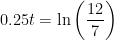
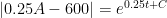
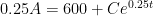
In yesterday’s post, I showed that the answer to this question was about 7.2 years. To obtain this answer, I started with the differential equation

which, given the initial condition 
Today, I’ll give some pedagogical thoughts about how this problem, and other similar problems inspired by financial considerations, could fit into a Precalculus course… and hopefully improve the financial literacy of high school students.

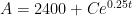
I’ve read many Precalculus books; not many of them include applying exponential functions to the paying off of credit-card debt (or a mortgage on a house or car). Of course, yesterday’s derivation was well above the comprehension level of students in Precalculus. However, there’s no reason why Precalculus students couldn’t be given the general formula
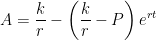
where 


Plugging in 


from which we find that it will take 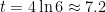
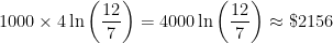
A natural follow-up question is “How much money actually was spent to pay off this debt?” By this point, the answer is quite easy: the lender paid 


When I teach this topic in differential equations, I let that answer sink in for a while. The original debt was only \$2000, but ultimately \$4300 needs to be paid over 7.2 years in order to pay off the debt.
The natural question is, “Why did it take so long?” Of course, the answer is that the debtor only paid the minimal amount — $50 per month, or $600 per year. It stands to reason that if extra money was paid each month, then the debt will be paid off faster at lesser expense.
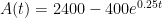
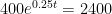
To give one example, let’s repeat the calculation if the debtor paid twice as much ($100 per month, or $1200 per year). Then the amount owed as a function of time would be

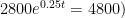
To find when the credit card will be paid off, we set 


That’s certainly a lot faster! Also, the amount that’s spent over that time is also considerably less:
So, along with being a good way to practice proficiency with exponential and logarithmic functions, this problem lends itself for students discovering some basic principles of financial literacy.
 be the amount of money on the credit card after
  years. Then there are two competing forces on the amount of money that will be owed in the future:
 per year.
 is actually a fraction. (In the derivation below, I will be a little sloppy with the arbitrary constant of integration for the sake of simplicity.)
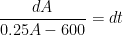


 , we use the initial condition


 . As part of this series, we considered the formula for continuous compound interest
 with solution
  . The meaning of the value of
  are
are  , while the units of
  . Therefore, the units of
  . So saying that there’s a “relative rate of growth of 10% per hour” makes total sense.
 .” But this is a horrible way to write this in ordinary English! After all, if we plug
  into the formula, we obtain


 and
and  , then
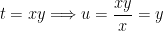
  is the inverse function of
  .
. , we define
 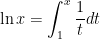 .
.


 is just a constant, we conclude


 . To this end, let’s apply implicit differentiation to this last equation:


 and
and  on their own after class.
 in Theorem 3. Alternatively, repeat the above argument for the inverse functions
  and
and  .
. . Suppose that
  has the following four properties:

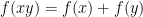 for all
 is continuous
 .
. .
. . (Please forgive the crudeness of this drawing; I’m only using Microsoft Paint.)
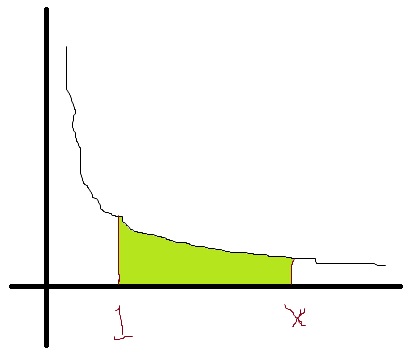
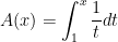
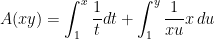
 is the right-hand limit, then
  is just the shaded area under the curve.
 is defined as an integral. That means that it must have…” Someone will usually volunteer, “A derivative.” I’ll respond, “That’s right. The Fundamental Theorem of Calculus says that this function is differentiable. So, if something is differentiable, then it also must be…” Someone will usually volunteer, “Continuous.” My response: “That’s right. So
  ?” After a moment of thought, someone will notice that
 .
. since the left and right endpoints of the integral are the same.
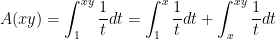 .
. to
to  has to be equal to the area from
  , is of course equal to
  .
. substitution:
 as the new variable of integration, and
  , how do we find
  ?” Students of course answer, “
 .” So I’ll follow up: “If
  , how do we find

 .
. .
.
 axis until the area under the hyperbola is equal to 1. Wherever this happens, that’s the number that we’ll call
  .
. , written more simply as
  has all of the properties of a logarithm and therefore must be a logarithmic function. The only catch is that we had to define
  , thus proving that
 , where


 . And this single case is simply handled through Property 1:
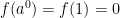
 . There is a natural way to approximate


 .
.
 .
.

 be a sequence of rational numbers that converges to
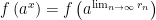
 .
. , this means that
 .
. .
.

 is a sequence that converges to
  . So, if we replace
  by
by  and
and  , we conclude that


 , even if


 , a negative rational number.
 ?” This leads to the proof of Case 3. I’ve found that it’s helpful to walk through this proof line by line in step with the case of
  , so that students can see how the steps of this more abstract proof correspond to the concrete example of
  .
. . Then


![2 = f(a^2) = f \left( \left[a^{2/3} \right]^3 \right)](https://s0.wp.com/latex.php?latex=2+%3D+f%28a%5E2%29+%3D+f+%5Cleft%28+%5Cleft%5Ba%5E%7B2%2F3%7D+%5Cright%5D%5E3+%5Cright%29&bg=ffffff&fg=000000&s=0&c=20201002)


 term?” The obvious correct answer:
 .
. ?” This leads to the proof of Case 2. I’ve found that it’s helpful to walk through this proof line by line in step with the case of
  , so that students can see how the steps of this more abstract proof correspond to the concrete example of
  .
. where
where  . Then
![m = f \left( \left[ a^{m/n} \right]^n \right)](https://s0.wp.com/latex.php?latex=m+%3D+f+%5Cleft%28+%5Cleft%5B+a%5E%7Bm%2Fn%7D+%5Cright%5D%5En+%5Cright%29&bg=ffffff&fg=000000&s=0&c=20201002)


 ?” Someone will usually suggest
  , and so I’ll write this as the next step:


 .
. , so that students can see how the steps of this more abstract proof correspond to the concrete example of
  .
.


 and
and  , then
  is the inverse function of
  .
. for all
  . That’s almost correct, and so I’ll ask if Property 2 is satisfied by this function. After a couple more moments of thought, someone will volunteer the correct answer,
  is Property 2.
 defined by
  must be equal to
  .
.