In my capstone class for future secondary math teachers, I ask my students to come up with ideas for engaging their students with different topics in the secondary mathematics curriculum. In other words, the point of the assignment was not to devise a full-blown lesson plan on this topic. Instead, I asked my students to think about three different ways of getting their students interested in the topic in the first place.
I plan to share some of the best of these ideas on this blog (after asking my students’ permission, of course).
This student submission again comes from my former student Caitlin Kirk. Her topic: how to engage Algebra II or Precalculus students when solving logarithmic equations.

B. Curriculum: How does this topic extend what your students should have learned in previous courses?
Logarithms are a topic that appears at multiple levels of high school math. In Algebra II, students are first introduced to logarithms when they are asked to identify graphs of parent functions including f (x) = logax. Later in the same class, they learn to formulate equations and inequalities based on logarithmic functions by exploring the relationship between logarithms and their inverses. From there, they can develop a definition of a logarithm.
Solving logarithmic equations extends what students learned about logarithms in Algebra II. Once a proper definition of logarithms has been established, along with a graphical foundation of logs, students learn to solve logarithmic equations. Properties of logarithms are used to expand, condense, and solve logarithms without a calculator in Pre Calculus. Practical applications of the logarithmic equation also follow from previous skills. Students learn to calculate the pH of a solution, decibel voltage gain, intensity of earthquakes measure on the Richter scale, depreciation, and the apparent loudness of sound using logarithms.
C. Culture: How has this topic appeared in the news?
One application of logarithmic equations is calculating the intensity of earthquakes measured on the Richter scale using the following equation:

where 

Reports of earthquake activity appear in the news often and are always accompanied by a measurement from the Richter scale. One such report can be found here: http://www.bbc.co.uk/news/world-asia-20638696. As the story says, a 7.3 magnitude earthquake struck off the coast of Japan in December of 2012, and created a small tsunami. There were six aftershocks of this quake whose Richter scale measurements are also given. The article also explains how Japan has been able to enact an early warning system that predicts the intensity of an earthquake before it causes damage. All of the calculations given in this story, and almost all others involving earthquakes, involves the use of the Richter scale logarithmic equation.
D. History: What are the contributions of various cultures to this topic?
The development of logarithms saw contributions from several different countries beginning with the Babylonians (2000-1600 BC) who developed the first known mathematical tables. They also introduced square multiplication in which they simply but accurately multiplied two numbers using only addition and subtraction. Michael Stifel, of Germany, was the first mathematician to use an exponent in 1544. He developed an early version of the logarithmic table containing integers and powers of 2. Perhaps the most important contribution to logarithms came from John Napier in Scotland in 1619. He, like the Babylonians, was working with on breaking multiplication, division, and root extraction down to only addition and subtraction. Therefore, he created the “logarithm” 

for which he wrote 
Napier’s definition of the logarithm led to the following logarithmic identities that are still taught today:


Henry Briggs, in England, published his work on logarithms in 1624, which included logarithms of 30,000 natural numbers to the 14th decimal place worked by hand! Shortly after, back in Germany, Johannes Kepler used a logarithmic scale on a Cartesian plane to create a linear graph the elliptical shape of the cosmos. In 1632, in Italy, Bonaventura Cavalieri published extensive tables of logarithms including the logs of trig functions (excluding cosine). Finally, Leonhard Euler made one of the most commonly known contributions to logarithms by making the number 


Logarithms were developed as a result of the contributions of many cultures spanning Europe and beyond, dating back over 4000 years.
 ,
, within some radius of convergence for all functions that commonly appear in the secondary mathematics curriculum.
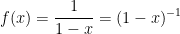 .
. ? Plugging in, we find
  .
. , we first find
  . Using the Chain Rule, we find
 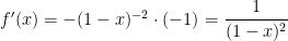 , so that
  .
. , so that
  .
. , so that
  .
. , so that
  .
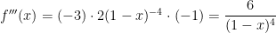
. , and this can be formally proved by induction.
 .
. , this series converges quickest for
  . Unlike the series for
  .
.
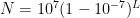
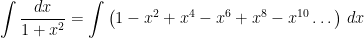
 and $r=x$. Also, as stated in precalculus, this series only converges if the common ratio satisfies $|r| < 1$, as before.
 . Let’s take the derivative of both sides (and ignore the fact that one should prove that differentiating this infinite series term by term is permissible). Since
 ,
, .
. with
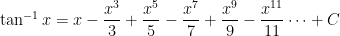
with  in the Taylor series in Step 5, obtaining


 :
:

 can be found by replacing

 in the Taylor series in Step 5, obtaining
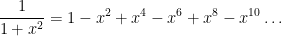


 .
. somehow simplfies as
  .
. distributes just as if
  was being multiplied by a constant. Other mistakes in this vein include
  and
and  .
. simplifies as
 simplifies as
  .
.