Confirming Einstein’s Theory of General Relativity With Calculus, Part 3: Method of Successive Approximations

In this series, I’m discussing how ideas from calculus and precalculus (with a touch of differential equations) can predict the precession in Mercury’s orbit and thus confirm Einstein’s theory of general relativity. The origins of this series came from a class project that I assigned to my Differential Equations students maybe 20 years ago.

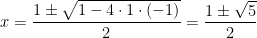
One technique that will be necessary for this confirmation is the method of successive approximations. This will be needed in the context of a differential equation; however, we can illustrate the concept by finding the roots of a polynomial. Consider the quadratic equation

$x^2 - x - 1 = 0$ .

(Naturally, we can solve for $x$ using the quadratic formula; more on that later.) To apply the method of successive approximation, we will rewrite this so that $x$ appears on the left side and some function of $x$ appears on the right side. I will choose

$x^2 = x + 1$ , or

$x = 1 + \displaystyle \frac{1}{x}$ .

Here’s the idea of the method of successive approximations to obtain a recursively defined sequence that (hopefully) convergence to a solution of this equation:

Start with an initial guess $x_0$ .
Plug $x_0$ into the right-hand side to get a new guess, $x_1$ .
Plug $x_1$ into the right-hand side to get a new guess, $x_2$ .
And repeat.

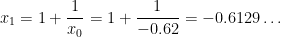
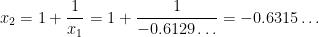
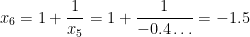
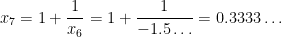
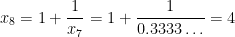
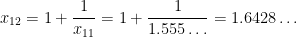
For example, suppose that we choose $x_0 = 1$ . Then

$x_1 = 1 + \displaystyle \frac{1}{x_0} = 1 + \displaystyle \frac{1}{1} = 2$

$x_2 = 1 + \displaystyle \frac{1}{x_1} = 1 + \displaystyle \frac{1}{2} = \displaystyle \frac{3}{2} = 1.5$

$x_3 = 1 + \displaystyle \frac{1}{x_2} = 1 + \displaystyle \frac{1}{3/2} = \displaystyle \frac{5}{3} \approx 1.667$

$x_4 = 1 + \displaystyle \frac{1}{x_3} = 1 + \displaystyle \frac{1}{5/3} = \displaystyle \frac{8}{5} = 1.6$

$x_5 = 1 + \displaystyle \frac{1}{x_4} = 1 + \displaystyle \frac{1}{8/5} = \displaystyle \frac{13}{8} = 1.625$

$x_6 = 1 + \displaystyle \frac{1}{x_5} = 1 + \displaystyle \frac{1}{13/8} = \displaystyle \frac{21}{13} \approx 1.615$

$x_7 = 1 + \displaystyle \frac{1}{x_6} = 1 + \displaystyle \frac{1}{21/13} = \displaystyle \frac{34}{21} \approx 1.619$

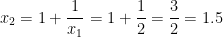
This sequence can be computed by entering $1$ into a calculator, then entering $1 + 1 \div \hbox{Ans}$ , and then repeatedly hitting the $=$ button.

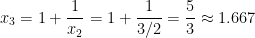
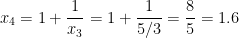
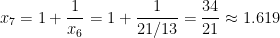
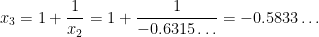
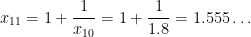
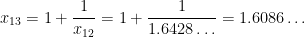
We see that the sequence appears to be converging to something, and that something is a root of the equation $x^2 - x - 1 = 0$ , which we now find via the quadratic formula:

$x = \displaystyle \frac{1 \pm \sqrt{1 - 4 \cdot 1 \cdot (-1)}}{2} = \frac{1 \pm \sqrt{5}}{2}$ .

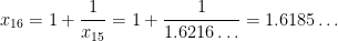
So it looks like the above sequence is converging to the positive root $(1 + \sqrt{5})/2 \approx 1.618$ .

(Parenthetically, you might notice that the Fibonacci sequence appears in the numerators and denominators of this sequence. As you might guess, that’s not a coincidence.)

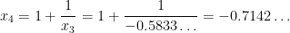
Like most numerical techniques, this method doesn’t always work like we think it would. Another solution is the negative root $(1 - \sqrt{5})/2 \approx -0.618$ . Unfortunately, if we start with a guess near this root, like $x_0 = -0.62$ , the sequence unexpectedly diverges from $-0.618\dots$ but eventually converges to the positive root $1.618\dots$ :

$x_1 = 1 + \displaystyle \frac{1}{x_0} = 1 + \displaystyle \frac{1}{-0.62} = -0.6129\dots$

$x_2 = 1 + \displaystyle \frac{1}{x_1} = 1 + \displaystyle \frac{1}{-0.6129\dots} = -0.6315\dots$

$x_3 = 1 + \displaystyle \frac{1}{x_2} = 1 + \displaystyle \frac{1}{-0.6315\dots} = -0.5833\dots$

$x_4 = 1 + \displaystyle \frac{1}{x_3} = 1 + \displaystyle \frac{1}{-0.5833\dots} = -0.7142\dots$

$x_5 = 1 + \displaystyle \frac{1}{x_4} = 1 + \displaystyle \frac{1}{-0.5833\dots} = -0.4$

$x_6 = 1 + \displaystyle \frac{1}{x_5} = 1 + \displaystyle \frac{1}{-0.4\dots} = -1.5$

$x_7 = 1 + \displaystyle \frac{1}{x_6} = 1 + \displaystyle \frac{1}{-1.5\dots} = 0.3333\dots$

$x_8 = 1 + \displaystyle \frac{1}{x_7} = 1 + \displaystyle \frac{1}{0.3333\dots} = 4$

$x_9 = 1 + \displaystyle \frac{1}{x_8} = 1 + \displaystyle \frac{1}{4} = 1.25$

$x_{10} = 1 + \displaystyle \frac{1}{x_9} = 1 + \displaystyle \frac{1}{1.25} = 1.8$

$x_{11} = 1 + \displaystyle \frac{1}{x_{10}} = 1 + \displaystyle \frac{1}{1.8} = 1.555\dots$

$x_{12} = 1 + \displaystyle \frac{1}{x_{11}} = 1 + \displaystyle \frac{1}{1.555\dots} = 1.6428\dots$

$x_{13} = 1 + \displaystyle \frac{1}{x_{12}} = 1 + \displaystyle \frac{1}{1.6428\dots} = 1.6086\dots$

$x_{14} = 1 + \displaystyle \frac{1}{x_{13}} = 1 + \displaystyle \frac{1}{1.6086\dots} = 1.6216\dots$

$x_{15} = 1 + \displaystyle \frac{1}{x_{14}} = 1 + \displaystyle \frac{1}{1.6216\dots} = 1.6166\dots$

$x_{16} = 1 + \displaystyle \frac{1}{x_{15}} = 1 + \displaystyle \frac{1}{1.6216\dots} = 1.6185\dots$

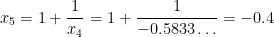
I should note that the method of successive approximations generally converges at a slower pace than Newton’s method. However, this method will be good enough when we use it to predict the precession in Mercury’s orbit.

Fibonacci joke

Source: https://www.facebook.com/Tysonism/photos/a.313776598684093/1921522124576191/?type=3&theater

Happy Fibonacci Day!

Today is 11/23, and 1, 1, 2, 3 are the first four terms of the Fibonacci sequence.

Courtesy Kris McCoy’s Pointless Math Fact of the Day.

My Favorite One-Liners: Part 28

In this series, I’m compiling some of the quips and one-liners that I’ll use with my students to hopefully make my lessons more memorable for them. Today’s quip is one that I’ll use when simple techniques get used in a complicated way.

Consider the solution of the linear recurrence relation

$Q_n = Q_{n-1} + 2 Q_{n-2}$ ,

where $F_0 = 1$ and $F_1 = 1$ . With no modesty, I call this one the Quintanilla sequence when I teach my students — the forgotten little brother of the Fibonacci sequence.

To find the solution of this linear recurrence relation, the standard technique — which is a pretty long procedure — is to first solve the characteristic equation, from $Q_n - Q_{n-1} - 2 Q_{n-2} = 0$ , we obtain the characteristic equation

$r^2 - r - 2 = 0$

This can be solved by any standard technique at a student’s disposal. If necessary, the quadratic equation can be used. However, for this one, the left-hand side simply factors:

$(r-2)(r+1) = 0$

$r=2 \qquad \hbox{or} \qquad r = -1$

(Indeed, I “developed” the Quintanilla equation on purpose, for pedagogical reasons, because its characteristic equation has two fairly simple roots — unlike the characteristic equation for the Fibonacci sequence.)

From these two roots, we can write down the general solution for the linear recurrence relation:

$Q_n = \alpha_1 \times 2^n + \alpha_2 \times (-1)^n$ ,

where $\alpha_1$ and $\alpha_2$ are constants to be determined. To find these constants, we plug in $n =0$ :

$Q_0 = \alpha_1 \times 2^0 + \alpha_2 \times (-1)^0$ .

To find these constants, we plug in $n =0$ :

$Q_0 = \alpha_1 \times 2^0 + \alpha_2 \times (-1)^0$ .

We then plug in $n =1$ :

$Q_1 = \alpha_1 \times 2^1 + \alpha_2 \times (-1)^1$ .

Using the initial conditions gives

$1 = \alpha_1 + \alpha_2$

$1 = 2 \alpha_1 - \alpha_2$

This is a system of two equations in two unknowns, which can then be solved using any standard technique at the student’s disposal. Students should quickly find that $\alpha_1 = 2/3$ and $\alpha_2 = 1/3$ , so that

$Q_n = \displaystyle \frac{2}{3} \times 2^n + \frac{1}{3} \times (-1)^n = \frac{2^{n+1} + (-1)^n}{3}$ ,

which is the final answer.

Although this is a long procedure, the key steps are actually first taught in Algebra I: solving a quadratic equation and solving a system of two linear equations in two unknowns. So here’s my one-liner to describe this procedure:

This is just an algebra problem on steroids.

Yes, it’s only high school algebra, but used in a creative way that isn’t ordinarily taught when students first learn algebra.

I’ll use this “on steroids” line in any class when a simple technique is used in an unusual — and usually laborious — way to solve a new problem at the post-secondary level.