In this series, I’m discussing how ideas from calculus and precalculus (with a touch of differential equations) can predict the precession in Mercury’s orbit and thus confirm Einstein’s theory of general relativity. The origins of this series came from a class project that I assigned to my Differential Equations students maybe 20 years ago.
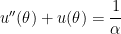
In this part of the series, we will show that if the motion of a planet around the Sun is expressed in polar coordinates 
where 


Part of the derivation of this governing differential equation will involve Newton’s Second Law

where 


where the components of the acceleration in the 


Unfortunately, our problem involves polar coordinates, and rewriting the acceleration vector in polar coordinates, instead of rectangular coordinates, is going to take some work.
Suppose that the position of the planet is 

where
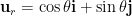
is a unit vector that points away from the origin. We see that this is a unit vector since

We also define
to be a unit vector that is perpendicular to 


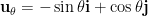
Computing the velocity and acceleration vectors in polar coordinates will have a twist that’s not experienced with rectangular coordinates since both
Furthermore,

These two equations will be needed in the derivation below.
We are now in position to express the velocity and acceleration of the orbiting planet in polar coordinates. Clearly, the position of the planet is 

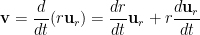
We now apply the Chain Rule to the second term:


Differentiating a second time with respect to time, and again using the Chain Rule, we find


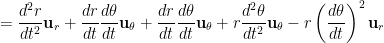
![= \displaystyle \left[ \frac{d^2r}{dt^2} - r \left(\frac{d\theta}{dt} \right)^2 \right] {\bf u}_r + \left[ 2\frac{dr}{dt} \frac{d\theta}{dt} + r \frac{d^2\theta}{dt^2} \right] {\bf u}_\theta](https://s0.wp.com/latex.php?latex=%3D+%5Cdisplaystyle+%5Cleft%5B+%5Cfrac%7Bd%5E2r%7D%7Bdt%5E2%7D+-++r+%5Cleft%28%5Cfrac%7Bd%5Ctheta%7D%7Bdt%7D+%5Cright%29%5E2+%5Cright%5D+%7B%5Cbf+u%7D_r+%2B+%5Cleft%5B+2%5Cfrac%7Bdr%7D%7Bdt%7D+%5Cfrac%7Bd%5Ctheta%7D%7Bdt%7D+%2B+r+%5Cfrac%7Bd%5E2%5Ctheta%7D%7Bdt%5E2%7D+%5Cright%5D+%7B%5Cbf+u%7D_%5Ctheta&bg=ffffff&fg=000000&s=0&c=20201002)
This will be needed in the next post, when we use both Newton’s Second Law and Newton’s Law of Gravitation, expressed in polar coordinates.
 ,
, is a constant. Of course, this can be written as
 ;
; in a form that depends only on


 .
. .
.


![= \displaystyle \frac{\ell}{mr^2} \frac{d}{d\theta} \left[ \frac{dr}{dt} \right]](https://s0.wp.com/latex.php?latex=%3D+%5Cdisplaystyle+%5Cfrac%7B%5Cell%7D%7Bmr%5E2%7D+%5Cfrac%7Bd%7D%7Bd%5Ctheta%7D+%5Cleft%5B+%5Cfrac%7Bdr%7D%7Bdt%7D+%5Cright%5D&bg=ffffff&fg=000000&s=0&c=20201002)
![= \displaystyle \frac{\ell}{mr^2} \frac{d}{d\theta} \left[ - \frac{\ell}{m} \frac{d}{d\theta} \left( \frac{1}{r} \right) \right]](https://s0.wp.com/latex.php?latex=%3D+%5Cdisplaystyle+%5Cfrac%7B%5Cell%7D%7Bmr%5E2%7D+%5Cfrac%7Bd%7D%7Bd%5Ctheta%7D+%5Cleft%5B+-+%5Cfrac%7B%5Cell%7D%7Bm%7D+%5Cfrac%7Bd%7D%7Bd%5Ctheta%7D+%5Cleft%28+%5Cfrac%7B1%7D%7Br%7D+%5Cright%29+%5Cright%5D&bg=ffffff&fg=000000&s=0&c=20201002)
![= \displaystyle - \frac{\ell^2}{m^2r^2} \frac{d}{d\theta} \left[ \frac{d}{d\theta} \left( \frac{1}{r} \right) \right]](https://s0.wp.com/latex.php?latex=%3D+%5Cdisplaystyle+-+%5Cfrac%7B%5Cell%5E2%7D%7Bm%5E2r%5E2%7D+%5Cfrac%7Bd%7D%7Bd%5Ctheta%7D+%5Cleft%5B+%5Cfrac%7Bd%7D%7Bd%5Ctheta%7D+%5Cleft%28+%5Cfrac%7B1%7D%7Br%7D+%5Cright%29+%5Cright%5D&bg=ffffff&fg=000000&s=0&c=20201002)
 .
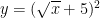
. if
if ![f(x) = \left[6x^2 + \sin 5x \right]^3](https://s0.wp.com/latex.php?latex=f%28x%29+%3D+%5Cleft%5B6x%5E2+%2B+%5Csin+5x+%5Cright%5D%5E3&bg=ffffff&fg=000000&s=0&c=20201002)
![f'(x) = 3 \left[6x^2 + \sin 5x \right]^2 \left(12x + [\cos 5x] \cdot 5 \right)](https://s0.wp.com/latex.php?latex=f%27%28x%29+%3D+3+%5Cleft%5B6x%5E2+%2B+%5Csin+5x+%5Cright%5D%5E2+%5Cleft%2812x+%2B+%5B%5Ccos+5x%5D+%5Ccdot+5+%5Cright%29&bg=ffffff&fg=000000&s=0&c=20201002)
![f'(x) = 3 \left[6x^2 + \sin 5x \right]^2 \left(12x + \cos 5x \right) \cdot 5](https://s0.wp.com/latex.php?latex=f%27%28x%29+%3D+3+%5Cleft%5B6x%5E2+%2B+%5Csin+5x+%5Cright%5D%5E2+%5Cleft%2812x+%2B+%5Ccos+5x+%5Cright%29+%5Ccdot+5&bg=ffffff&fg=000000&s=0&c=20201002)
 at the end of the derivative. Students can so easily get into the rhythm of just multiplying by the derivative of the inside that they can forget where the derivative of the inside should be placed.
 for positive and negative integers
  , the trigonometric function, and
  . They also know the Product and Quotient Rules.
 . Then

 .
. . Then

 . Then

 . Then


 in the first example as $\latex 3 \times 2$.
 and
and  . In other words, there’s a significant front-end investment of time as students discover the Chain Rule, but applying the Chain Rule generally moves along quite quickly once it’s been discovered.