Mathematical Allusions in Shantaram (Part 1)

I recently finished the novel Shantaram, by Gregory David Roberts. As I’m not a professional book reviewer, let me instead quote from the Amazon review:

Crime and punishment, passion and loyalty, betrayal and redemption are only a few of the ingredients in Shantaram, a massive, over-the-top, mostly autobiographical novel. Shantaram is the name given Mr. Lindsay, or Linbaba, the larger-than-life hero. It means “man of God’s peace,” which is what the Indian people know of Lin. What they do not know is that prior to his arrival in Bombay he escaped from an Australian prison where he had begun serving a 19-year sentence. He served two years and leaped over the wall. He was imprisoned for a string of armed robberies performed to support his heroin addiction, which started when his marriage fell apart and he lost custody of his daughter. All of that is enough for several lifetimes, but for Greg Roberts, that’s only the beginning.

He arrives in Bombay with little money, an assumed name, false papers, an untellable past, and no plans for the future. Fortunately, he meets Prabaker right away, a sweet, smiling man who is a street guide. He takes to Lin immediately, eventually introducing him to his home village, where they end up living for six months. When they return to Bombay, they take up residence in a sprawling illegal slum of 25,000 people and Linbaba becomes the resident “doctor.” With a prison knowledge of first aid and whatever medicines he can cadge from doing trades with the local Mafia, he sets up a practice and is regarded as heaven-sent by these poor people who have nothing but illness, rat bites, dysentery, and anemia. He also meets Karla, an enigmatic Swiss-American woman, with whom he falls in love. Theirs is a complicated relationship, and Karla’s connections are murky from the outset.

While it was a cracking good read, what struck me particularly were the surprising mathematical allusions that the author used throughout the novel. In this mini-series, I’d like to explore the ones that I found.

In this first installment, the narrator describes a life-or-death situation as he is being choked:

He was a hard man. He didn’t give up. His hands squeezed tighter. My neck was strong and the muscles were well developed, but I knew he had the strength to kill me. My hand reached, groping for the pistol in my pocket. I had to shoot him. I had to kill him. That was all right. I didn’t care. The air in my lungs was spent, and my brain was exploding in Mandelbrot whirls of colored light, and I was dying, and I wanted to kill him.
Shantaram, Chapter 25

Someone being choked to death might be prosaically described as “seeing stars,” but the author instead to choose the more vivid imagery of “exploding in Mandelbrot whirls of colored light.” The Mandelbrot set is a fractal that solves a famous mathematical problem:

And the Mandelbrot set is quite colorful and complex, which might indeed be a better description than “seeing stars” of what might be going through someone’s mind when being choked to death. Although somewhat dated, here’s my favorite Mandelbrot zoom video:

My Mathematical Magic Show: Part 11

A couple years ago, I learned the 27-card trick, which is probably the most popular trick in my current repertoire. In this first video, Matt Parker performs this trick as well as the 49-card trick.

Here’s a quick explanation from the American Mathematical Society for how the magician performs this trick. In short, the magician needs to do some mental arithmetic quickly.

The 27 card trick is based on the ternary number system, sometimes called the base 3 system.

Suppose the volunteer chooses a card and also chooses the number 18. You want to make her chosen card move to the 18th position in the deck, which means you need 17 cards above it. You first need to express 17 in base 3, writing it as a three digit number. For the procedure used in this trick, it’s also handy to write the digits in backward order: 1s digit first, 3s digit second, and 9s digit last. In this backward base 3 notation 17 becomes 221, since 17 = 2×3⁰ + 2×3¹ + 1×3².

With the understanding that 2 = bottom, 1 = middle, and 0 = top, the number 17 becomes “bottom-bottom-middle.”

Now deal the cards into three piles. The subject identifies the pile containing her card. That pile should be placed at the position indicated by the 1s digit, which is 2, or bottom. After picking up the three piles with the pile containing the chosen card on the bottom, deal the cards a second time into three piles. This time place the pile containing the chosen card in the position indicated by the 3s digit, which is also 2, or bottom. Finally, after placing the pile containing the subject’s card on the bottom, deal the cards into three piles for a third time. When picking up the piles, this time place the pile containing her card in the position indicated by the 9s digit, which is 1, or middle. Deal out 17 cards. The 18th will be her card.

Making a schematic picture of the deck, like Matt does in his second video [below], should convince you that this procedure does precisely what is claimed. But there is no substitute for actually doing it—take 27 cards and try it!

Of course this procedure will work regardless of which position the subject chooses, for her choice is always a number between 1 and 27. This means you need between 0 and 26 cards on top of it, and in base 3 we have 0 = 000 (top-top-top) and 26 = 222 (bottom-bottom-bottom). Every possible position that the subject can choose corresponds to a unique base 3 representation.

In general, if you deal a pack of n^k cards into n piles, have the subject identify the pile that contains her card, and repeat this procedure k times, you can place her card at any desired position in the deck. The idea is the same: Subtract one from the desired position number, and convert the result to base n as a k digit number. The ones digit of this number tells you where to place the packet containing her card after the first deal (n – 1 = bottom, 0 = top), and the procedure continues for the remaining deals.

In Mathematics, Magic and Mystery (Dover, 1956), Martin Gardner discusses the long history and many variations of this effect. See Chapter 3, “From Gergonne to Gargantua.”

In this Numberphile video, Matt Parker explains why the trick works.

My Mathematical Magic Show: Part 10

This magic trick is an optical illusion instead of a pure magic trick, but it definitely is a crowd-pleaser. This illusion is called Sugihara’s Impossible Cylinder:

This is actually a mathematical magic trick. As detailed by David Richeson in Math Horizons, there is a fair amount of math that goes into creating this unique shape. He also provided this interacted Geogebra applet as well as a printable pdf file for creating this illusion.

Confirming Einstein’s Theory of General Relativity With Calculus, Part 9: Pedagogical Thoughts

At long last, we have reached the end of this series of posts.

The derivation is elementary; I’m confident that I could have understood this derivation had I seen it when I was in high school. That said, the word “elementary” in mathematics can be a bit loaded — this means that it is based on simple ideas that are perhaps used in a profound and surprising way. Perhaps my favorite quote along these lines was this understated gem from the book Three Pearls of Number Theory after the conclusion of a very complicated proof in Chapter 1:

You see how complicated an entirely elementary construction can sometimes be. And yet this is not an extreme case; in the next chapter you will encounter just as elementary a construction which is considerably more complicated.

Here are the elementary ideas from calculus, precalculus, and high school physics that were used in this series:

Physics
- Conservation of angular momentum
- Newton’s Second Law
- Newton’s Law of Gravitation
Precalculus
- Completing the square
- Quadratic formula
- Factoring polynomials
- Complex roots of polynomials
- Bounds on $\cos \theta$ and $\sin \theta$
- Period of $\cos \theta$ and $\sin \theta$
- Zeroes of $\cos \theta$ and $\sin \theta$
- Trigonometric identities (Pythagorean, sum and difference, double-angle)
- Conic sections
- Graphing in polar coordinates
- Two-dimensional vectors
- Dot products of two-dimensional vectors (especially perpendicular vectors)
- Euler’s equation
Calculus
- The Chain Rule
- Derivatives of $\cos \theta$ and $\sin \theta$
- Linearizations of $\cos x$ , $\sin x$ , and $1/(1-x)$ near $x \approx 0$ (or, more generally, their Taylor series approximations)
- Derivative of $e^x$
- Solving initial-value problems
- Integration by $u-$ substitution

While these ideas from calculus are elementary, they were certainly used in clever and unusual ways throughout the derivation.

I should add that although the derivation was elementary, certain parts of the derivation could be made easier by appealing to standard concepts from differential equations.

One more thought. While this series of post was inspired by a calculation that appeared in an undergraduate physics textbook, I had thought that this series might be worthy of publication in a mathematical journal as an historical example of an important problem that can be solved by elementary tools. Unfortunately for me, Hieu D. Nguyen’s terrific article Rearing Its Ugly Head: The Cosmological Constant and Newton’s Greatest Blunder in The American Mathematical Monthly is already in the record.

Confirming Einstein’s Theory of General Relativity With Calculus, Part 8: Second- and Third-Order Approximations

In this series, I’m discussing how ideas from calculus and precalculus (with a touch of differential equations) can predict the precession in Mercury’s orbit and thus confirm Einstein’s theory of general relativity. The origins of this series came from a class project that I assigned to my Differential Equations students maybe 20 years ago.

In this series, we found an approximate solution to the governing initial-value problem

$u''(\theta) + u(\theta) = \displaystyle \frac{1}{\alpha} + \delta [u(\theta)]^2$

$u(0) = \displaystyle \frac{1 + \epsilon}{\alpha}$

$u'(0) = 0$ ,

where $u = \displaystyle \frac{1}{r}$ , $\displaystyle \frac{1}{\alpha} = \frac{GMm^2}{\ell^2}$ , $\delta = \displaystyle \frac{3GM}{c^2}$ , $G$ is the gravitational constant of the universe, $m$ is the mass of the planet, $M$ is the mass of the Sun, $\ell$ is the constant angular momentum of the planet, $\epsilon$ is the eccentricity of the orbit, and $c$ is the speed of light.

We used the following steps to find an approximate solution.

Step 0. Ignore the general-relativity contribution and solve the simpler initial-value problem

$u_0''(\theta) + u_0(\theta) = \displaystyle \frac{1}{\alpha}$

$u_0(0) = \displaystyle \frac{1 + \epsilon}{\alpha}$

$u_0'(0) = 0$ ,

which is a zeroth-order approximation to the real initial-value problem. We found that the solution of this differential equation is

$u_0(\theta) = \displaystyle \frac{1 + \epsilon \cos \theta}{\alpha}$ ,

which is the equation of an ellipse in polar coordinates.

Step 1. Solve the initial-value problem

$u_1''(\theta) + u_1(\theta) = \displaystyle \frac{1}{\alpha} + \delta [u_0(\theta)]^2$

$u_1(0) = \displaystyle \frac{1 + \epsilon}{\alpha}$

$u_1'(0) = 0$ ,

which partially incorporates the term due to general relativity. This is a first-order approximation to the real differential equation. After much effort, we found that the solution of this initial-value problem is

$u_1(\theta) = \displaystyle \frac{1 + \epsilon \cos \theta}{\alpha} + \frac{\delta}{\alpha^2} + \frac{\delta \epsilon^2}{2\alpha^2} + \frac{ \delta\epsilon}{\alpha^2} \theta \sin \theta - \frac{ \delta \epsilon^2}{6\alpha^2} \cos 2\theta - \frac{\delta(3+\epsilon^2)}{3\alpha^2} \cos \theta$ .

For large values of $\theta$ , this is accurately approximated as:

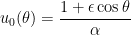
$u_1(\theta) \approx \displaystyle \frac{1 + \epsilon \cos \theta}{\alpha} + \frac{ \delta\epsilon}{\alpha^2} \theta \sin \theta$ ,

which can be further approximated as

$u_1(\theta) \approx \displaystyle \frac{1}{\alpha} \left[ 1 + \epsilon \cos \left( \theta - \frac{\delta \theta}{\alpha} \right) \right]$ .

From this expression, the precession in a planet’s orbit due to general relativity can be calculated.

Roughly 20 years ago, I presented this application of differential equations at the annual meeting of the Texas Section of the Mathematical Association of America. After the talk, a member of the audience asked what would happen if we did this procedure yet again to find a second-order approximation. In other words, I was asked to consider…

Step 2. Solve the initial-value problem

$u_2''(\theta) + u_2(\theta) = \displaystyle \frac{1}{\alpha} + \delta [u_1(\theta)]^2$

$u_2(0) = \displaystyle \frac{1 + \epsilon}{\alpha}$

$u_2'(0) = 0$ .

It stands to reason that the answer should be an even more accurate approximation to the true solution $u(\theta)$ .

I didn’t have an immediate answer for this question, but I can answer it now. Letting Mathematica do the work, here’s the answer:

Yes, it’s a mess. The term in red is $u_0(\theta)$ , while the term in yellow is the next largest term in $u_1(\theta)$ . Both of these appear in the answer to $u_2(\theta)$ .

The term in green is the next largest term in $u_2(\theta)$ , with the highest power of $\theta$ in the numerator and the highest power of $\alpha$ in the denominator. In other words,

$u_2(\theta) \approx \displaystyle \frac{1 + \epsilon \cos \theta}{\alpha} + \frac{ \delta\epsilon}{\alpha^2} \theta \sin \theta -\frac{\delta^2 \epsilon}{2\alpha^3} \theta^2 \cos \theta$ .

How does this compare to our previous approximation of

$u(\theta) \approx \displaystyle \frac{1}{\alpha} \left[ 1 + \epsilon \cos \left( \theta - \frac{\delta \theta}{\alpha} \right) \right]$ ?

Well, to a second-order Taylor approximation, it’s the same! Let

$f(x) = \displaystyle \frac{1}{\alpha} \left[ 1 + \epsilon \cos \left( \theta - x \right) \right]$ .

Expanding about $x = 0$ and treated $\theta$ as a constant, we find

$f(x) \approx f(0) + f'(0) x + \displaystyle \frac{f''(0)}{2} x^2 = \displaystyle \frac{1}{\alpha} \left[ 1 + \epsilon \cos \left( \theta\right) \right] + \frac{\epsilon}{\alpha} x \sin \theta - \frac{\epsilon}{2\alpha} x^2 \cos \theta$ .

Substituting $x = \displaystyle \frac{\delta \theta}{\alpha}$ yields the above approximation for $u_2(\theta)$ .

Said another way, proceeding to a second-order approximation merely provides additional confirmation for the precession of a planet’s orbit.

Just for the fun of it, I also used Mathematica to find the solution of Step 3:

Step 2. Solve the initial-value problem

$u_3''(\theta) + u_3(\theta) = \displaystyle \frac{1}{\alpha} + \delta [u_2(\theta)]^2$

$u_3(0) = \displaystyle \frac{1 + \epsilon}{\alpha}$

$u_3'(0) = 0$ .

I won’t copy-and-paste the solution from Mathematica; unsurpisingly, it’s really long. I will say that, unsurprisingly, the leading terms are

$u_3(\theta) \approx \displaystyle \frac{1 + \epsilon \cos \theta}{\alpha} + \frac{ \delta\epsilon}{\alpha^2} \theta \sin \theta -\frac{\delta^2 \epsilon}{2 \alpha^3} \theta^2 \cos \theta -\frac{\delta^3 \epsilon}{6\alpha^4} \theta^3 \sin \theta$ .

I said “unsurprisingly” because this matches the third-order Taylor polynomial of our precession expression. I don’t have time to attempt it, but surely there’s a theorem to be proven here based on this computational evidence.

Happy Pythagoras Day!

I’m posting one day early this week to wish everyone a Happy Pythagoras Day! Today is 7/25/24 (or 25/7/24 in other parts of the world), and $25^2 = 7^2 + 24^2$ .

Bonus points if you can figure out (without Googling) when the next Pythagoras Day will be.

Confirming Einstein’s Theory of General Relativity With Calculus, Part 7e: Computing Precession

We have shown that under general relativity, the motion of a planet around the Sun precesses by

$\phi = \displaystyle \frac{6\pi GM}{ac^2 (1-\epsilon^2)} \qquad \hbox{radians per orbit}$ ,

where $a$ is the semi-major axis of the planet’s orbit, $\epsilon$ is the orbit’s eccentricity, $G$ is the gravitational constant of the universe, $M$ is the mass of the Sun, and $c$ is the speed of light.

Notice that for $\phi$ to be as observable as possible, we’d like $a$ to be as small as possible and $\epsilon$ to be as large as possible. By a fortunate coincidence, the orbit of Mercury — the closest planet to the sun — has the most elliptical orbit of the eight planets.

Here are the values of the constants for Mercury’s orbit in the SI system:

$G = 6.6726 \times 10^{-11} \qquad \hbox{N-m}^2/\hbox{kg}^2$
$M = 1.9929 \times 10^{30} \qquad \hbox{kg}$
$a = 5.7871 \times 10^{10} \qquad \hbox{m}$
$c = 2.9979 \times 10^{8} \qquad \hbox{m/s}$
$\epsilon = 0.2056$
$T = 0.2408 \qquad \hbox{years}$

The last constant, $T$ , is the time for Mercury to complete one orbit. This isn’t in the SI system, but using Earth years as the unit of time will prove useful later in this calculation.

Using these numbers, and recalling that $1 ~ \hbox{N} = 1 ~ \hbox{kg-m/s}^2$ , we find that

$\phi = \displaystyle \frac{6\pi \times 6.6726 \times 10^{-11} ~ \hbox{m}^3/(\hbox{kg-s}^2) \times 1.9929 \times 10^{30} ~ \hbox{kg}}{5.7871 \times 10^{10} ~ \hbox{m} \times (2.9979 \times 10^{8} ~ \hbox{m/s})^2 \times (1-(0.2408)^2)} \approx 5.03 \times 10^{-7}$ .

Notice that all of the units cancel out perfectly; this bit of dimensional analysis is a useful check against careless mistakes.

Again, the units of $\phi$ are in radians per Mercury orbit, or radians per 0.2408 years. We now convert this to arc seconds per century:

$\phi \approx 5.03 \times 10^{-7} \displaystyle \frac{\hbox{radians}}{\hbox{0.2408 years}} \times \frac{180 ~\hbox{degrees}}{\pi ~ \hbox{radians}} \times \frac{3600 ~ \hbox{arc seconds}}{1 ~ \hbox{degree}} \times \frac{100 ~ \hbox{years}}{1 ~ \hbox{century}}$

$\phi = 43.1 \displaystyle \frac{\hbox{arc seconds}}{\hbox{century}}$ .

This indeed matches the observed precession in Mercury’s orbit, thus confirming Einstein’s theory of relativity.

This same computation can be made for other planets. For Venus, we have the new values of $a = 1.0813 \times 10^{11} ~ \hbox{m}$ , $\epsilon = 0.0068$ , and $T = 0.6152 ~ \hbox{years}$ . Repeating this calculation, we predict the precession in Venus’s orbit to be 8.65” per century. Einstein made this prediction in 1915, when the telescopes of the time were not good enough to measure the precession in Venus’s orbit. This only happened in 1960, 45 years later and 5 years after Einstein died. Not surprisingly, the precession in Venus’s orbit also agrees with general relativity.

Confirming Einstein’s Theory of General Relativity With Calculus, Part 7d: Predicting Precession IV

We have shown that the motion of a planet around the Sun, expressed in polar coordinates $(r,theta)$ with the Sun at the origin, under general relativity is

$u(\theta) \approx \displaystyle \frac{1}{\alpha} \left[ 1 + \epsilon \cos \left( \theta - \frac{\delta \theta}{\alpha} \right) \right]$ ,

where $u = \displaystyle \frac{1}{r}$ , $\alpha = a(1-\epsilon^2)$ , $a$ is the semi-major axis of the planet’s orbit, $\epsilon$ is the orbit’s eccentricity, $\delta = \displaystyle \frac{3GM}{c^2}$ , $G$ is the gravitational constant of the universe, $m$ is the mass of the planet, $M$ is the mass of the Sun, $P$ is the planet’s perihelion, $\ell$ is the constant angular momentum of the planet, and $c$ is the speed of light.

The above function $u(\theta)$ is maximized (i.e., the distance from the Sun $r(\theta)$ is minimized) when $\displaystyle \cos \left( \theta - \frac{\delta \theta}{\alpha} \right)$ is as large as possible. This occurs when $\theta - \displaystyle \frac{\delta \theta}{\alpha}$ is a multiple of $2\pi$ .

Said another way, the planet is at its closest point to the Sun when $\theta = 0$ . One orbit later, the planet returns to its closest point to the Sun when

$\theta - \displaystyle \frac{\delta \theta}{\alpha} = 2\pi$

$\theta \displaystyle\left(1 - \frac{\delta}{\alpha} \right) = 2\pi$

$\theta = 2\pi \displaystyle\frac{1}{1 - (\delta/\alpha)}$

We now use the approximation

$\displaystyle \frac{1}{1-x} \approx 1 + x \qquad \hbox{if} \qquad x \approx 0$ ;

this can be demonstrated by linearization, Taylor series, or using the first two terms of the geometric series $1 + x + x^2 + x^3 + \dots$ . With this approximation, the closest approach to the Sun in the next orbit occurs when

$\theta = 2\pi \displaystyle\left(1 + \frac{\delta}{\alpha} \right) = 2\pi + \frac{2\pi \delta}{\alpha}$ ,

which is coterminal with the angle

$\phi = \displaystyle \frac{2\pi \delta}{\alpha}$ .

Substituting $\alpha = a(1-\epsilon^2)$ and $\delta = \displaystyle \frac{3GM}{c^2}$ , we see that the amount of precession per orbit is

$\phi = \displaystyle 2 \pi \frac{3GM}{c^2} \frac{1}{a(1-\epsilon^2)} = \frac{6\pi G M}{ac^2(1-\epsilon^2)}$ .

The units of $\phi$ are radians per orbit. In the next post, we will use Mercury’s data to find $\phi$ in seconds of arc per century.

Confirming Einstein’s Theory of General Relativity With Calculus, Part 7c: Predicting Precession III

We have shown that the motion of a planet around the Sun, expressed in polar coordinates $(r,theta)$ with the Sun at the origin, under general relativity is

$u(\theta) \approx \displaystyle \frac{1}{\alpha} \left[ 1 + \epsilon \cos \left( \theta - \frac{\delta \theta}{\alpha} \right) \right]$ ,

where $u = \displaystyle \frac{1}{r}$ , $\displaystyle \frac{1}{\alpha} = \frac{GMm^2}{\ell^2}$ , $\epsilon = \displaystyle \frac{\alpha - P}{P}$ , $\delta = \displaystyle \frac{3GM}{c^2}$ , $G$ is the gravitational constant of the universe, $m$ is the mass of the planet, $M$ is the mass of the Sun, $P$ is the planet’s perihelion, $\ell$ is the constant angular momentum of the planet, and $c$ is the speed of light.

We notice that the orbit of a planet under general relativity looks very, very similar to the orbit under Newtonian physics:

$u(\theta) \approx \displaystyle \frac{1}{\alpha} \left[ 1 + \epsilon \cos \theta \right]$ ,

so that

$r(\theta) = \displaystyle \frac{\alpha}{1 + \epsilon \cos \theta}$ .

As we’ve seen, this describes an elliptical orbit, normally expressed in rectangular coordinates as

$\displaystyle \frac{(x-h)^2}{a^2} + \frac{y^2}{b^2} = 1$ ,

with semimajor axis along the $x-$ axis. In particular, for an elliptical orbit, the planet’s closest approach to the Sun occurs at $\theta = 0$ :

$r(0) = \displaystyle \frac{\alpha}{1 + \epsilon \cos 0} = \frac{\alpha}{1 + \epsilon}$ ,

and the planet’s further distance from the Sun occurs at $\theta = \pi$ :

$r(\pi) = \displaystyle \frac{\alpha}{1 + \epsilon \cos \pi} = \frac{\alpha}{1 - \epsilon}$ .

Therefore, the length $2a$ of the major axis of the ellipse is the sum of these two distances:

$2a = \displaystyle \frac{\alpha}{1 + \epsilon} + \frac{\alpha}{1 - \epsilon}$

$2a = \displaystyle \frac{\alpha(1-\epsilon) + \alpha(1+\epsilon)}{(1 + \epsilon)(1 - \epsilon)}$

$2a= \displaystyle \frac{2\alpha}{1 - \epsilon^2}$

$a = \displaystyle \frac{\alpha}{1 - \epsilon^2}$ .

Said another way, $\alpha = a(1-\epsilon^2)$ . This is a far more convenient formula for computing $\alpha$ than $\alpha = \displaystyle \frac{\ell^2}{GMm^2}$ , as the values of $a$ (the semi-major axis) and $\epsilon$ (the eccentricity of the orbit) are more accessible than the angular momentum $\ell$ of the planet’s orbit.

In the next post, we finally compute the precession of the orbit.

Confirming Einstein’s Theory of General Relativity With Calculus, Part 7b: Predicting Precession II

We have shown that the motion of a planet around the Sun, expressed in polar coordinates $(r,\theta)$ with the Sun at the origin, under general relativity is

$u(\theta) \approx \displaystyle \frac{1 + \epsilon \cos \theta}{\alpha} + \frac{ \delta\epsilon}{\alpha^2} \theta \sin \theta$ ,

We will now simplify this expression, using the facts that $\delta$ is very small and $\alpha$ is quite large, so that $\delta/\alpha$ is very small indeed. We will use the two approximations

$\cos x \approx 1 \qquad \hbox{and} \qquad \sin x \approx x \qquad \hbox{if} \qquad x \approx 0$ ;

these approximations can be obtained by linearization or else using the first term of the Taylor series expansions of $\cos x$ and $\sin x$ about $x = 0$ .

We will also need the trig identity

$\cos(\theta_1 - \theta_2) = \cos \theta_1 \cos \theta_2 + \sin \theta_1 \sin \theta_2$ .

With these tools, we can now simplify $u(\theta)$ :

$u(\theta) \approx \displaystyle \frac{1 + \epsilon \cos \theta}{\alpha} + \frac{ \delta\epsilon}{\alpha^2} \theta \sin \theta$

$= \displaystyle \frac{1}{\alpha} \left[1 + \epsilon \cos \theta + \frac{ \delta\epsilon}{\alpha} \theta \sin \theta \right]$

$= \displaystyle \frac{1}{\alpha} \left[1 + \epsilon \left(\cos \theta + \frac{ \delta}{\alpha} \theta \sin \theta \right) \right]$

$= \displaystyle \frac{1}{\alpha} \left[1 + \epsilon \left(\cos \theta \cdot 1 + \sin \theta \cdot \frac{ \delta \theta}{\alpha} \right) \right]$

$\approx \displaystyle \frac{1}{\alpha} \left[1 + \epsilon \left(\cos \theta \cdot \cos \frac{\delta \theta}{\alpha} + \sin \theta \cdot \sin \frac{ \delta \theta}{\alpha} \right) \right]$

$\approx \displaystyle \frac{1}{\alpha} \left[1 + \epsilon \cos \left( \theta - \frac{\delta \theta}{\alpha} \right) \right]$ .