In my capstone class for future secondary math teachers, I ask my students to come up with ideas for engaging their students with different topics in the secondary mathematics curriculum. In other words, the point of the assignment was not to devise a full-blown lesson plan on this topic. Instead, I asked my students to think about three different ways of getting their students interested in the topic in the first place.

I plan to share some of the best of these ideas on this blog (after asking my students’ permission, of course).

This student submission again comes from my former student Maranda Edmonson. Her topic, from Geometry: deriving the Pythagorean theorem.

D. History: What are the contributions of various cultures to this topic?

Legend has it that Pythagoras was so happy about the discovery of his most famous theorem that he offered a sacrifice of oxen. His theorem states that “the area of the square built upon the hypotenuse of a right triangle is equal to the sum of the areas of the squares upon the remaining sides.” It is likely, though, that the ancient Babylonians and Egyptians knew the result much earlier than Pythagoras, but it is uncertain how they originally demonstrated the proof. As for the Greeks, it is likely that methods similar to Euclid’s Elements were used. Also, though there are many proofs of the Pythagorean Theorem, one came from the contemporary Chinese civilization found in the Arithmetic Classic of the Gnoman and the Circular Paths of Heaven, a Chinese text containing formal mathematical theories.

http://jwilson.coe.uga.edu/emt669/student.folders/morris.stephanie/emt.669/essay.1/pythagorean.html

E. Technology: How can technology be used to effectively engage students with this topic?

The following link is for a video that not only engages students from the very beginning by playing the Mission: Impossible theme and giving students a mission – “should they choose to accept it” – but that has great information. It begins with a short engagement, as stated before, and goes into a little bit of history about Pythagoras and the Pythagoreans. It then briefly describes what the Pythagorean Theorem is before the commentator says, “Does it have applications in our lives today?” At this point (2:43 in the video), it would be beneficial to stop the video and let students discuss where they could use the theorem. The rest of the video simply shows some examples of how the Pythagorean Theorem is used on sailboats, inclined planes, and televisions. It would be up to the teacher whether or not to show the last five minutes of the video to show students these examples, but they could take notes on these examples as they are worked out on the screen.

http://digitalstorytelling.coe.uh.edu/movie_mathematics_02.html

B. Applications: How can this topic be used in your students’ future courses in mathematics or science?

After students learn the Pythagorean Theorem in their Geometry classes, they will use it throughout their mathematical careers. They will use it specifically in Pre-Calculus when they are learning about the unit circle. The theorem is fundamental to proving the basic identities in Trigonometry. It is also used in some of the trigonometric identities, aptly named the Pythagorean Identities based on the nature of their derivation.

In Physics, the kinetic energy of an object is

$\displaystyle \frac{1}{2} (\hbox{mass})(\hbox{velocity})^2$ .

But, in terms of energy, energy at 500 mph = energy at 300 mph + energy at 400 mph. This equation means that, with the energy used to accelerate something at 500 mph, two other objects could use that same energy to be accelerated to 300 mph and 400 mph. Looks like a Pythagorean triple, right? The theorem is also used in Computer Science with processing time. Other examples are found in the link below.

http://betterexplained.com/articles/surprising-uses-of-the-pythagorean-theorem/

Why does 0.999… = 1? (Part 5)

Here’s one more way of convincing students that $0.\overline{9} = 1$ . Here’s the idea: how far apart are the two numbers?

First off, since $1 \ge 0.\overline{9}$ , we know that $1 - \overline{9} \ge 0$ .

Of course, we know that $1-0.9 = 0.1$ . Since $0.\overline{9}$ must lie between $0.9$ and $1$ , we know that $1 - 0.\overline{9}$ must be less than $0.1$ .

Second, we know that $1-0.99 = 0.01$ . Since $0.\overline{9}$ must lie between $0.99$ and $1$ , we know that $1 - 0.\overline{9}$ must be less than $0.01$ .

Third, we know that $1-0.999 = 0.001$ . Since $0.\overline{9}$ must lie between $0.999$ and $1$ , we know that $1 - 0.\overline{9}$ must be less than $0.001$ .

By the same reasoning, we conclude that

$0 \le 1 - 0.\overline{9} < \displaystyle \frac{1}{10^n}$

for every integer $n$ . What’s the only number that’s greater than or equal to $0$ and less than every decimal of the form $0.00\dots001$ ? Clearly, the only such number is $0$ . Therefore,

$1 - 0.\overline{9} = 0$ , or $0.\overline{9} = 1$ .

I like this approach because it really gets at the heart of the difference between integers $\mathbb{Z}$ and real numbers $\mathbb{R}$ . For integers, there is always an integer to the immediate left and to the immediate right. In other words, if you give me any integer (say, $15$ ), I can tell you the largest integer that’s less than your number (in our example, $14$ ) and the smallest integer that’s bigger than your number ( $16$ ).

Real numbers, however, do not have this property. There is no real number to the immediate right of $0$ . This is easy to prove by contradiction. Suppose $x > 0$ is the real number to the immediate left of $0$ . That means that there are no real numbers between $0$ and $x$ . However, $x/2$ is bigger than $0$ and less than $x$ , providing the contradiction.

(For what it’s worth, the above proof doesn’t apply to the set of integers $\mathbb{Z}$ since $x/2$ doesn’t have to be an integer.)

By the same logic — visually, you can imagine reflecting the number line across the point $x = 0.5$ — there is no number to the immediate left of $1$ . So while $0.\overline{9}$ would appear to be to the immediate left of $1$ , they are in reality the same point.

Why does 0.999… = 1? (Part 4)

In this series, I discuss some ways of convincing students that $0.999\dots = 1$ and that, more generally, a real number may have more than one decimal representation even though a decimal representation corresponds to only one real number. This can be a major conceptual barrier for even bright students to overcome. I have met a few math majors within a semester of graduating — that is, they weren’t dummies — who could recite all of these ways and were perhaps logically convinced but remained psychologically unconvinced.

Method #5. This is a proof by contradiction; however, I think it should be convincing to a middle-school student who’s comfortable with decimal representations. Also, perhaps unlike Methods #1-4, this argument really gets to the heart of the matter: there can’t be a number in between $0.999\dots$ and $1$ , and so the two numbers have to be equal.

In the proof below, I’m deliberating avoiding the explicit use of algebra (say, letting $x$ be the midpoint) to make the proof accessible to pre-algebra students.

Suppose that $0.999\dots < 1$ . Then the midpoint of $0.999\dots$ and $1$ has to be strictly greater than $0.999\dots$ , since

$\displaystyle \frac{0.999\dots + 1}{2} > \displaystyle \frac{0.999\dots + 0.999\dots}{2} = 0.999\dots$

Similarly, the midpoint is strictly less than $1$ :

$\displaystyle \frac{0.999\dots + 1}{2} < \displaystyle \frac{1 +1}{2} =1$

(For the sake of convincing middle-school students, a number line with three tick marks — for $0.999\dots$ , $1$ , and the midpoint — might be more believable than the above inequalities.)

So what is the decimal representation of the midpoint? Since the midpoint is less than $1$ , the decimal representation has to be $0.\hbox{something}$ Furthermore, the midpoint does not equal $0.999\dots$ . That means, somewhere in the decimal representation of the midpoint, there’s a digit that’s not equal to $9$ . In other words, the midpoint has to have one of the following 9 forms:

midpoint = $0.999\dots 990 \, \_ \, \_ \dots$

midpoint = $0.999\dots 991 \, \_ \, \_ \dots$

midpoint = $0.999\dots 992 \, \_ \, \_ \dots$

midpoint = $0.999\dots 993 \, \_ \, \_ \dots$

midpoint = $0.999\dots 994 \, \_ \, \_ \dots$

midpoint = $0.999\dots 995 \, \_ \, \_ \dots$

midpoint = $0.999\dots 996 \, \_ \, \_ \dots$

midpoint = $0.999\dots 997 \, \_ \, \_ \dots$

midpoint = $0.999\dots 998 \, \_ \, \_ \dots$

In any event, $9$ is the largest digit. That means that, no matter what, the midpoint is less than $0.999\dots$ , contradicting the fact that the midpoint is larger than $0.999\dots$ (if $0.999\dots < 1$ ).

Why does 0.999… = 1? (Part 3)

Method #4. This is a direct method using the formula for an infinite geometric series… and hence will only be convincing to students if they’re comfortable with using this formula. By definition,

$0.999\dots = \displaystyle \frac{9}{10} + \frac{9}{100} + \frac{9}{1000} + \dots$

This is an infinite geometric series. Its first term is $\displaystyle \frac{9}{10}$ , and the common ratio needed to go from one term to the next term is $\displaystyle \frac{1}{10}$ . Therefore,

$0.999\dots = \displaystyle \frac{ \displaystyle \frac{9}{10}}{ \quad \displaystyle 1 - \frac{1}{10} \quad}$

$0.999\dots = \displaystyle \frac{ \displaystyle \frac{9}{10}}{ \quad \displaystyle \frac{9}{10} \quad}$

$0.999\dots = 1$

Why does 0.999… = 1? (Part 2)

Methods #2 and #3 are indirect methods. We start with a decimal representation that we know and end with $0.999\dots$ .

Method #2. This technique should be accessible to any student who can do long division. With long division, we know full well that

$\displaystyle \frac{1}{3} = 0.333\dots$

Multiply both sides by $3$ :

$\displaystyle 3 \times \frac{1}{3} = 3 \times 0.333\dots$

$\displaystyle 1 = 0.999\dots$

Though not logically necessary, this method could be reinforced for students by also considering

$\displaystyle 1 = 9 \times \frac{1}{9} = 9 \times 0.111\dots = 0.999\dots$

Method #3. With long division, we know full well that

$\displaystyle \frac{1}{3} = 0.333\dots \quad$ and $~ \quad \displaystyle \frac{2}{3} = 0.666\dots$

Add them together:

$\displaystyle \frac{1}{3} + \frac{2}{3} = 0.333\dots + 0.666\dots$

$\displaystyle 1 = 0.999\dots$

Though not logically necessary, this method could be reinforced for students by also considering any (or all) of the following:

$1 = \displaystyle \frac{1}{9} + \frac{8}{9} = 0.111\dots + 0.888\dots = 0.999\dots$

$1 = \displaystyle \frac{2}{9} + \frac{7}{9} = 0.222\dots + 0.777\dots = 0.999\dots$

$1 = \displaystyle \frac{4}{9} + \frac{5}{9} = 0.444\dots + 0.555\dots = 0.999\dots$

Why does 0.999… = 1? (Part 1)

Our decimal number system is so wonderful that it’s often taken for granted. (If you doubt me, try multiplying $12$ and $61$ or finding an $18\%$ tip on a restaurant bill using only Roman numerals.)

However, there’s one little quirk about our numbering system that some students find quite unsettling:

If a number has a terminating decimal representation, then the same number also has a second different terminating decimal representation. (However, a number that does not have a terminating decimal representation does not have a second representation.)

Stated another way, a decimal representation corresponds to a unique real number. However, a real number may not have a unique decimal representation.

Some (perhaps many) students find such equalities to be unsettling at first glance, and for good reason. They’d prefer to think that there is a one-to-one correspondence to the set of real numbers and the set of decimal representations. Stated more simply, students are conditioned to think that if two number look different (like $24$ and $25$ ), then they ought to be different.

However, there’s a subtle difference between a number and a numerical representation. The number $1$ is defined to be the multiplicative identity in our system of arithmetic. However, this number has two different representations in our numbering system: $1$ and $0.999\dots$ . (Not to mention its representation in the numbering systems of the ancient Romans, Babylonians, Mayans, etc.)

As usual, let $[0,1]$ be the set of real numbers from $0$ to $1$ (inclusive), and let $D$ be the set of decimal representations of the form $0.d_1 d_2 d_3 \dots$ . Then there’s clearly a function $f : D \to \mathbb{R}$ , defined by

$f(0.d_1 d_2 d_3\dots) = \displaystyle \sum_{i=1}^\infty \frac{d_n}{10^n}$

If I want to give my students a headache, I’ll ask, “In Calculus II, you saw that some series converge and some series diverge. So what guarantee do we have that this series actually converges?” (The convergence of the right series can be verified using the Direct Comparsion Test, the fact that $d_i \le 9$ , and the formula for an infinite geometric series.)

In the language of mathematics: Using the completeness axiom, it can be proven (though no student psychologically doubts this) that $f$ maps $D$ onto $[0,1]$ . In other words, every decimal representation corresponds to a real number, and every real number has a decimal representation. However, the function $f$ is a surjection but not a bijection. In other words, a real number may have more than one decimal representation.

This is a big conceptual barrier for some students — even really bright students — to overcome. They’re not used to thinking that two different decimal expansions can actually represent the same number.

The two most commonly shown equal but different decimal representations are $0.999\dots = 1$ . Other examples are

$0.125 = 0.124999\dots$

$3.458 = 3.457999 \dots$

In this series, I will discuss some ways of convincing students that $0.999\dots = 1$ . That said, I have met a few math majors within a semester of graduating — that is, they weren’t dummies — who could recite all of these ways and were perhaps logically convinced but remained psychologically unconvinced. The idea that two different decimal representations could mean the same number just remained too high of a conceptual barrier for them to hurdle.

Method #1. This first technique is accessible to any algebra or pre-algebra student who’s comfortable assigning a variable to a number. We convert the decimal representation to a fraction using something out of the patented Bag of Tricks. If students aren’t comfortable with the first couple of steps (as in, “How would I have thought to do that myself?”), I tell my usual tongue-in-cheek story: Socrates gave the Bag of Tricks to Plato, Plato gave it to Aristotle, it passed down the generations, my teacher taught the Bag of Tricks to me, and I teach it to my students.

Let $x =0.999\dots$ . Multiply $x$ by $10$ , and subtract:

$10x = 9.999\dots$

$x = 0.999\dots$

$\therefore (10-1)x = 9$

$x =1$

$0.999\dots = 1$

Factoring the time

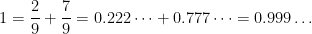
True story: one way that I commit large numbers to (hopefully) short-term memory is by factoring. If I take the time to factor a big number, then I can usually remember it for a little while.

This approach has occasional disadvantages. For example, I now have stuck in my brain the completely useless information that, many years ago, my seat at a Texas Rangers ballgame was somewhere in Section 336 (which is $6 \times 7 \times 8$ ).

Source: http://www.xkcd.com/247/

Engaging students: Introducing variables and expressions

I plan to share some of the best of these ideas on this blog (after asking my students’ permission, of course).

This student submission again comes from my former student Caitlin Kirk. Her topic, from Pre-Algebra: introducing variables and expressions.

To keep track of some of the coldest things in the universe, scientist use the Kelvin temperature scale that begins at 0 Kelvin, or Absolute Zero. Nothing can ever be colder than Absolute Zero because at this temperature, all motion stops. The table below shows some typical temperatures of different systems in the universe.

Table of Cold Places

Temp.(K)	Location
183	Vostok, Antarctica
160	Phobos- a moon of Mars
128	Europa in the summer
120	Moon at night
88	Miranda surface temp.
81	Enceladus in the summer
70	Mercury at night
55	Pluto in the summertime
50	Dwarf Planet Quaoar
33	Pluto in the wintertime
1	Boomerang Nebula
0	ABSOLUTE ZERO

You are probably already familiar with the Celsius (C) and Fahrenheit (F) temperature scales. The two formulas below show how to switch from degrees-C to degrees-F.

$C = \frac{5}{9} (F-32)$

$F = \frac{9}{5} C + 32$

Because the Kelvin scale is related to the Celsius scale, we can also convert from Celsius to Kelvin (K) using the equation:

$K = 273 + C$

Problems

Use these three equations to convert between the three temperature scales:

Problem 1: 212 F converted to K

Problem 2: 0 K converted to F

Problem 3: 100 C converted to K

Problem 4: Two scientists measure the daytime temperature of the moon using two different instruments. The first instrument gives a reading of +107 C while the second instrument gives +221 F.

a. What are the equivalent temperatures on the Kelvin scale?

b. What is the average daytime temperature on the Kelvin scale?

Problem 5: Humans can survive without protective clothing in temperatures ranging from 0 F to 130 F. In what, if any, locations from the table above can humans survive?

Solutions

Problem 1: First convert to C: C = 5/9 (212-32) = +100 C. Then convert from C to K: K = 273 + 100 = 373 Kelvin.

Problem 2: First convert to Celsius: 0 = 273 + C so C = -273. Then convert from C to F: F = 9/5 (-273) + 32 = -459 Fahrenheit.

Problem 3: K = 273 – 100 = 173 Kelvin.

Problem 4:

a. 107 C becomes K = 273 + 107 = 380 Kelvin. 221 F becomes C = 5/9(221-32) = 105 C, and so K = 273 + 105 = 378 Kelvin.

b. (380 + 378)/2 = 379 Kelvin

Problem 5:

First convert 0 F and 130 F to Celsius so that the conversion to Kelvin is quicker. 0 F becomes C = 5/9(0-32) = -18 C (rounded to the nearest degree) and 130 F becomes C = 5/9 (130-32) = 54 C (rounded to the nearest degree).

Next, convert -18 C and 54 C to Kelvin. -18 C becomes K = 273-18 = 255 and 54 C becomes k = 273 + 54 = 327 K.

None of the locations on the table have temperatures between 255 K and 327 K, therefore humans could not survive in any of these space locations.

A. How can this topic be used in your students’ future courses in mathematics or science?

This topic is one of the first experiences students have with algebra. Since algebra is the point from which students dive into more advanced mathematics, this topic will be used in many different areas of future mathematics. After mastering the use of one variable, with the basic operations of addition, subtraction, multiplication, and division, students will be introduced to the use of more than one variable. They may be asked to calculate the area of a solid whose perimeter is given and whose side lengths are unknown variables. Or in a more advanced setting, they may be asked to calculate how much money will be in a bank account after five years of interest compounded continuously. In fact, the use of variables is present and important in every mathematics class from Algebra I through Calculus and beyond. There very well may never be a day in a mathematics students’ life where they will not see a variable after variables have been introduced.

B. How does this topic extend what your students should have learned in previous courses?

In basic arithmetic, probably in elementary or early middle school math classes, students learn how to do calculations with numbers using the four basic operations of addition, subtraction, multiplication and division. They also learn simple applications of these basic operations by calculating the area and perimeter of a rectangle, for example. Introducing variables and expressions is a continuation of those same ideas except that one or more of the numbers is now an unknown variable. Students can rely on the arithmetic skills they already possess when learning this introduction to algebra with variables and expressions.

Students are familiar with calculating the area and perimeter of figures like the one on the left before they are introduced to variables. Later, they may see the same figure with the addition of a variable, as shown on the right. The addition of the variable will come with new instructions as well.

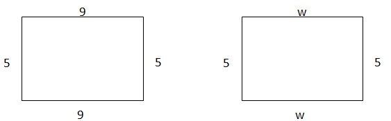
The difficulty of problems using variables is determined by the information given in the problems. For instance, the problem on the right can be a one step equation if an area and perimeter are given so that students only need to solve for w. The difficulty can be increased by giving only a perimeter so that students must solve for w and then for the area.

Engaging students: Computing the determinant of a matrix

I plan to share some of the best of these ideas on this blog (after asking my students’ permission, of course).

This student submission again comes from my former student Caitlin Kirk. Her topic: computing the determinant of a matrix.

B. Curriculum: How does this topic extend what your students should have learned in previous courses?

Students learn early in their mathematical careers how to calculate the area of simple polygons such as triangles and parallelograms. They learn by memorizing formulas and plugging given values into the formulas. Matrices, and more specifically the determinant of a matrix, can be used to do the same thing.

For example, consider a triangle with vertices $(1,2)$ , $(3, -4)$ , and $(-2,3)$ . The traditional method for finding the area of this circle would be to use the distance formula to find the length of each side and the height before plugging and chugging with the formula $A = \frac{1}{2} bh$ . Matrices can be used to compute the same area in fewer steps using the fact that the area of a triangle the absolute value of one-half times the determinant of a matrix containing the vertices of the triangle as shown below.

First, put the vertices of the triangle into a matrix using the x-values as the first column and the corresponding y-values as the second column. Then fill the third column with 1’s as shown:

Next, compute the determinant of the matrix and multiply it by ½ (because the traditional area formula for a triangle calls for multiplying by ½ to account for the fact that a triangle is half of a rectangle, it is necessary to keep the ½ here also) as shown:

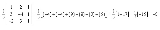Obviously, the area of a triangle cannot be negative. Therefore it is necessary to take the absolute value of the final answer. In this case $|-8| = 8$ , making the area positive eight instead of negative eight.

The same idea can be applied to extend students knowledge of the area of other polygons such as a parallelogram, rectangle, or square. Determinants of matrices are a great extension of the basic mathematical concept of area that students will have learned in previous courses.

D. History: What are the contributions of various cultures to this topic?

The history of matrices can be traced to four different cultures. First, Babylonians as early as 300 BC began attempting to solve simultaneous linear equations like the following:

There are two fields whose total area is eighteen hundred square yards. One produces grain at the rate of two-thirds of a bushel per square yard while the other produces grain at the rate of on-half a bushel per square yard. If the total yield is eleven hundred bushels, what is the size of each field?

While the Babylonians at this time did not actually set up matrices or calculate any determinants, they laid the framework for later cultures to do so by creating systems of linear equations.

The Chinese, between 200 BC and 100 BC, worked with similar systems and began to solve them using columns of numbers that resemble matrices. One such problem that they worked with is given below:

There are three types of corn, of which three bundles of the first, two of the second, and one of the third make 39 measures. Two of the first, three of the second and one of the third make 34 measures. And one of the first, two of the second and three of the third make 26 measures. How many measures of corn are contained of one bundle of each type?

Unlike the Babylonians, the Chinese answered this question using their version of matrices, called a counting board. The counting board functions the same way as modern matrices but is turned on its side. Modern matrices write a single equation in a row and the next equation in the next row and so forth. Chinese counting boards write the equations in columns. The counting board below corresponds to the question above:

1 2 3

2 3 2

3 1 1

26 34 39

They then used what we know as Gaussian elimination and back substitution to solve the system by performing operations on the columns until all but the bottom row contains only zeros and ones. Gaussian elimination with back substitution did not become a well known method until the early 19^th century, however.

Next, in 1683, the Japanese and Europeans simultaneously saw the discovery and use of a determinant, though the Japanese published it first. Seki, in Japan, wrote Method of Solving the Dissimulated Problems which contains tables written in the same manner as the Chinese counting board. Without having a word to correspond to his calculations, Seki calculated the determinant and introduced a general method for calculating it based on examples. Using his methods, Seki was able to find the determinants of 2×2, 3×3, 4×4, and 5×5 matrices.

In the same year in Europe, Leibniz wrote that the system of equations below:

$10+11x+12y=0$

$20+21x+22y=0$

$30+31x+32y=0$

has a solution because

$(10 \times 21 \times 32)+(11 \times 22 \times 30)+(12 \times 20 \times 31)=(10 \times 22 \times 31)+(11 \times 20 \times 32)+(12 \times 21 \times 30)$ .

This is the exact condition under which the matrix representing the system has a determinant of zero. Leibniz was the first to apply the determinant to finding a solution to a linear system. Later, other European mathematicians such as Cramer, Bezout, Vandermond, and Maclaurin, refined the use of determinants and published rules for how and when to use them.

Source: http://www-history.mcs.st-and.ac.uk/HistTopics/Matrices_and_determinants.html

B. Curriculum: How can this topic be used in you students’ future courses in mathematics or science?

Calculating the determinant is used in many lessons in future mathematics courses, mainly in algebra II and pre-calculus. The determinant is the basis for Cramer’s rule that allows a student to solve a system of linear equations. This leads to other methods of solving linear systems using matrices such as Gaussian elimination and back substitution. It can also be used in determining the invertibility of matrices. A matrix whose determinant is zero does not have an inverse. Invertibility of matrices determines what other properties of matrix theory a given matrix will follow. If students were to continue pursuing math after high school, understanding determinants is essential to linear algebra.

Mean Green Math

Dating pools

Engaging students: Deriving the Pythagorean theorem

Why does 0.999… = 1? (Part 5)

Why does 0.999… = 1? (Part 4)

Why does 0.999… = 1? (Part 3)

Why does 0.999… = 1? (Part 2)

Why does 0.999… = 1? (Part 1)

Factoring the time

Engaging students: Introducing variables and expressions

Engaging students: Computing the determinant of a matrix