Source: http://www.xkcd.com/1248/
Source: http://www.xkcd.com/1248/
In this series of posts, I provide a deeper look at common applications of exponential functions that arise in an Algebra II or Precalculus class. In the previous posts in this series, I considered financial applications, radioactive decay, and Newton’s Law of Cooling.
Today, I discuss the logistic growth model, which describes how an infection (like a disease, a rumor, or advertise) spreads in a population. In yesterday’s post, I described an in-class demonstration that engages students while also making the following formula believable:

I’d like to discuss some observations about this somewhat complicated function that will make producing its graph easier. The first two observations are within reach of Precalculus students.
1. Let’s figure out the 

In other words, the number 
2. Let’s figure out the limiting value as 

As expected, all 

3. Let’s now figure out the point of inflection. Ordinarily, points of inflection are found by setting the second derivative equal to zero. Though this can be done for the function 
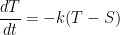
The good news is that the points of inflection can be found quite simply using the governing differential equation, which is
Let’s take the derivative of both sides, remembering that 
So the second derivative is equal to zero when either 


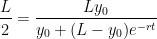
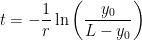
This suggests that, as the infection spreads throughout a population, the curve changes concavity at the time that half of the population becomes infected. In other words, the infection spreads fastest throughout the population at the time when half of the population has been infected.
The time at which the point of inflection occurs can be found by setting 
This technique for finding the points of inflection directly from the differential equation is possible whenever the differential equation is autonomous, which loosely means that the independent variable does not appear on the right-hand side.
In this series of posts, I provide a deeper look at common applications of exponential functions that arise in an Algebra II or Precalculus class. In the previous posts in this series, I considered financial applications, radioactive decay, and Newton’s Law of Cooling.
Today, I introduce the logistic growth model, which describes how an infection (like a disease, a rumor, or advertise) spreads in a population. For example:

or
Sources: http://www.xkcd.com/1220/ and http://www.xkcd.com/1235/
In yesterday’s post, I described an in-class demonstration that engages students while also making the following formula believable:

Where does this formula come from? Suppose that a disease is spreading in a population of size 
![A(t) [ L - A(t) ]](https://s0.wp.com/latex.php?latex=A%28t%29+%5B+L+-+A%28t%29+%5D+&bg=ffffff&fg=000000&s=0&c=20201002)
![A'(t) = c A(t) [ L - A(t) ]](https://s0.wp.com/latex.php?latex=A%27%28t%29+%3D+c+A%28t%29+%5B+L+-+A%28t%29+%5D&bg=ffffff&fg=000000&s=0&c=20201002)
where 


The good news is that this differential equation can be solved using separation of variables, just like the governing differential equations for continuous compound interest, paying off credit card debt, radioactive decay, and Newton’s Law of Cooling. The bad news is that it’s a lot harder to calculate the required integrals! After all, the right-hand side, after distributing, has a term containing 
Solving this differential equation is a bit tedious, and I don’t feel particularly obligated to re-invent the wheel since it can be found several places on the Internet. Suffice it to say that integration by partial fractions and some very tricky algebra is necessary to solve for
Wikipedia: http://en.wikipedia.org/wiki/Logistic_function#In_ecology:_modeling_population_growth
MathWorld: http://mathworld.wolfram.com/LogisticEquation.html
In this series of posts, I provide a deeper look at common applications of exponential functions that arise in an Algebra II or Precalculus class. In the previous posts in this series, I considered financial applications, radioactive decay, and Newton’s Law of Cooling.
Today, I introduce the logistic growth model, which describes how an infection (like a disease, a rumor, or advertise) spreads in a population. Before I actually present the formula to my students, I usually perform a 8- to 10-minute demonstration to convince students that the formula actually works. This demonstration works well with between 15 and 45 students; I have personally not attempted this demo with a class larger than 45.
I wish I could take credit for the idea behind this demonstration. I’m afraid I can’t remember who told me the idea behind this demo about 15 years ago, but I’m thankful to him or her for this idea, as I’ve used it with great success over the years when teaching Precalculus and even when teaching Differential Equations.
Here’s the demonstration:
1. The class period before the demo, I ask my students to bring their calculators to class.
2. On the day of the demo, I prepare slips of paper with the numbers 1, 2, 3, etc. I hand these to my students as they take their seats before class starts (and, as needed, to students who arrive late).
3. I tell the class that we’re going to model how a rumor gets spread. On the chalkboard, I write down the numbers 0, 1, 2, …, up to 
4. I point out that, at time 0, only one person has heard the rumor…. me. I’m person number 0 (confirming the popular belief of my students). So I’ll cross out the 0 on the board and mark on a table that only one person has heard the rumor so far. (Here’s the spreadsheet that I’ve used to keep track of this information while simultaneously making a graph of the data: logisitic).
5. I begin to spread the rumor. To spread the rumor, I use my calculator to get a random number between 


For example, in the figure below, I would tell that person #35 of my class of 37 students was the next to hear the rumor. (If my random number is 0, I’ll privately cheat and get until I get a random number other than 0. I only permit the possibility of cheating on the first step so that the data fits the predicted curve as accurately as possible.)
 6. At this point, I’ll X out the number of the next person to hear the rumor (in this case, 35), and I then ask how many people have heard the rumor. Obviously, two people have heard the rumor. So I’ll note on the table that two people have heard the rumor after one step.
7. Now we repeat the process. I get a new random number, and I ask the first student to pull out his/her calculator to get a random number too. But there’s an important rule: if you get a number that’s already been called, that’s OK. This models what really happens when a rumor (or disease) spreads in a population — it’s perfectly possible to hear the rumor twice.
8. We repeat the process — X’ing out numbers that have been previously called and students calling out the next person to hear the rumor — until the entire class hears the rumor. At some point, it becomes easiest to ask students to only call out if they get a number that hasn’t been called yet. Invariably, there’s always one person at the end who hasn’t heard the rumor yet, and this student is often the subject of some good-natured ribbing. Eventually, a chart like the following is produced.

9. Students immediately see that this is a different type of function than pure exponential growth. It actually does start off looking like exponential growth, but at some point the curve levels off. This makes sense because there’s a limiting value of 
10. The punchline is that the spreadsheet secretly computes the actual curve predicted by the logistic growth model. The numbers are actually located in column C, which is conveniently hidden beneath the graph. The function is
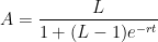
where 


I never expect the curve to exactly fit the data, but it should come pretty close. After this fairly dramatic revelation, my students are completely sold that the mathematics that I’m about to show them actually works.
In this series of posts, I provide a deeper look at common applications of exponential functions that arise in an Algebra II or Precalculus class. In the previous posts in this series, I considered financial applications. In today’s post, I’ll discuss Newton’s Law of Cooling, which describes how quickly a hot object cools in a room at constant temperature. (This law is not to be confused with Newton’s Three Laws of Motion.)
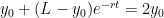
While Newton’s Law of Cooling is easy to state, not many high school teachers are aware of the physical principles from which they arise. The basic idea is that the rate at which a hot object cools is proportional to the difference between its current temperature and the surrounding temperature. After solving the appropriate differential equation, the temperature 

where 

Of course, students in Algebra II or Precalculus (or high school physics) are usually not ready to understand this derivation using calculus. Instead, they are typically given the final formula and are expected to use this formula to solve problems. Still, I think it’s important for the teacher of Algebra II or Precalculus to be aware of how the origins of this formula, as it only requires mathematics that’s only a year or two away in these students’ mathematical development.
This is the third application of exponential functions considered in this series; the previous two were continuous compound interest and radioactive decay. Unlike these previous two applications, Newton’s Law of Cooling can actually be demonstrated in class to engage students. All that’s required is the appropriate classroom technology and a standard-issue temperature probe.This stands in sharp contrast to the previous applications of exponential functions considered in this series. While students can easily envision making money via compound interest, no one will actually give them the money during class. And certainly I don’t encourage performing a real demonstration of radioactive decay with, say uranium-235, during class time! (There are ways of simulating radioactive decay using M&Ms or other manipulatives, however.)
A simple Google search yields thousands of webpages describes multiple classroom activities for Newton’s Law of Cooling. Some activities merely require collecting data and performing a regression fit to an exponential curve; such an activity would be appropriate for middle-school students. Other activities are more explicit about using Newton’s Law of Cooling. Here’s a sampling:
These links are aimed at a students at a variety of levels. Indeed, it’s possible to use a graphing calculator to plot the numerical derivative 
In this series of posts, I provide a deeper look at common applications of exponential functions that arise in an Algebra II or Precalculus class. In the previous posts in this series, I considered financial applications. In today’s post, I’ll discuss Newton’s Law of Cooling, which describes how quickly a hot object cools in a room at constant temperature. (This law is not to be confused with Newton’s Three Laws of Motion.)
While Newton’s Law of Cooling is easy to state, not many high school teachers are aware of the physical principles from which they arise. The basic idea is that the rate at which a hot object cools is proportional to the difference between its current temperature and the surrounding temperature. In other words, in a room at a temperature of $70^\circ$F, a very hot object at $270^\circ$F will cool twice as fast than when its temperature drops to $170^\circ$F.
The above paragraph can be rewritten as a differential equation. Let $T(t)$ be the temperature of the object at time 
where
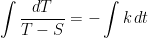
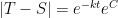
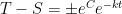
This differential equation can be solved in several ways, including separation of variables (below, I’ll be sloppy with the constant of integration for the sake of simplicity):
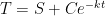
To solve for the constant, we usually use the initial condition 
Plugging back in, we obtain the final answer
Of course, students in Algebra II or Precalculus (or high school physics) are usually not ready to understand this derivation using calculus. Instead, they are typically given the final formula and are expected to use this formula to solve problems. Still, I think it’s important for the teacher of Algebra II or Precalculus to be aware of how the origins of this formula, as it only requires mathematics that’s only a year or two away in these students’ mathematical development.
The careful reader will notice that this derivation essentially parallels the previous derivations for continuous compound interest and for radioactive decay. In other words, these phenomena from apparently different realms of life have similar solutions because the governing differential equations are very similar.
For more information, see http://io9.com/prepare-to-have-your-mind-blown-by-a-balloon-and-a-mini-1565303363?utm_campaign=socialflow_io9_facebook&utm_source=io9_facebook&utm_medium=socialflow
See also Smarter Every Day’s channel: http://www.youtube.com/user/destinws2
I thought something on the lighter side would be appropriate today… like rapping about the Large Hadron Collider at CERN, where the Higgs boson was (tentatively) discovered.
The following report from CNN (http://www.cnn.com/2014/03/24/world/asia/malaysia-airlines-satellite-tracking/index.html?hpt=hp_t1; the video from CNN can be found at http://www.cnn.com/video/data/2.0/video/world/2014/03/24/lead-foreman-satellite-data-mh370.cnn.html) discusses in layman’s terms how applied mathematicians were able to track the final moments of Flight 370. Here are the relevant paragraphs:
The mathematics-based process used by Inmarsat and the UK’s Air Accidents Investigation Branch (AAIB) to reveal the definitive path was described by McLaughlin as “groundbreaking.”
“We’ve done something new,” he said.
Here’s how the process works in a nutshell: Inmarsat officials and engineers were able to determine whether the plane was flying away or toward the satellite’s location by expansion or compression of the satellite’s signal.
What does expansion or compression mean? You may have heard about something called the Doppler effect.
“If you sit at a train station and you listen to the train whistle — the pitch of the whistle changes as it moves past. That’s exactly what we have,” explained CNN Meteorologist Chad Myers,who has studied Doppler technology. “It’s the Doppler effect that they’re using on this ping or handshake back from the airplane. They know by nanoseconds whether that signal was compressed a little — or expanded — by whether the plane was moving closer or away from 64.5 degrees — which is the latitude of the orbiting satellite.”
Each ping was analyzed for its direction of travel, Myers said. The new calculations, McLaughlin said, underwent a peer review process with space agency experts and contributions by Boeing.
It’s possible to use this analysis to determine more specifically the area where the plane went down, Myers said. “Using trigonometry, engineers are capable of finding angles of flight.”
My understanding is that even though the pings from a satellite to the plane and back were occurring, even though the plane’s location was not being transmitted. From the Doppler shift of those pings, the plane’s trajectory could be reconstructed.
Someday, for teaching purposes, I hope that a formal write-up of this procedure is published. The details will probably be over the heads of most students, but this is a eye-catching, though indescribably tragic, example of how mathematics can be creatively used to solve a mystery.

This is one of most creative diagrams that I’ve ever seen: the depth of various solar system gravity wells. A large version of this image can be accessed at http://xkcd.com/681_large/.
From the fine print:
Each well is scaled so that rising out of a physical well of that depth — in constant Earth surface gravity — would take the same energy as escaping from that planet’s gravity in reality.
Depth =
It takes the same amount of energy to launch something on an escape trajectory away from Earth as it would to launch is 6,000 km upward under a constant
Earth gravity. Hence, Earth’s well is 6,000 km deep.
Here’s some more details about the above formula.
Step 1. The escape velocity from the surface of a spherical planet is

where 


Step 2. Suppose that a rocket moves at constant velocity upward near the surface of the earth. Then the force exerted by the rocket exactly cancel the force of gravity, so that

where 

The depth formula used in the comic is then found by equating these two expressions and solving for
![A' = r A [ L - A] = r L A - r A^2](https://s0.wp.com/latex.php?latex=A%27+%3D+r+A+%5B+L+-+A%5D+%3D+r+L+A+-+r+A%5E2&bg=ffffff&fg=000000&s=0&c=20201002)


![A'(t) = \displaystyle \frac{r}{L} A(t) [ L - A(t) ]](https://s0.wp.com/latex.php?latex=A%27%28t%29+%3D+%5Cdisplaystyle+%5Cfrac%7Br%7D%7BL%7D+A%28t%29+%5B+L+-+A%28t%29+%5D&bg=ffffff&fg=000000&s=0&c=20201002)
![A'(t) = r A(t) \displaystyle \left[1 - \frac{A(t)}{L} \right]](https://s0.wp.com/latex.php?latex=A%27%28t%29+%3D+r+A%28t%29+%5Cdisplaystyle+%5Cleft%5B1+-+%5Cfrac%7BA%28t%29%7D%7BL%7D+%5Cright%5D&bg=ffffff&fg=000000&s=0&c=20201002)