Solving Problems Submitted to MAA Journals (Part 5d)

The following problem appeared in Volume 96, Issue 3 (2023) of Mathematics Magazine.

Evaluate the following sums in closed form:

$f(x) = \displaystyle \sum_{n=0}^\infty \left( \cos x - 1 + \frac{x^2}{2!} - \frac{x^4}{4!} \dots + (-1)^{n-1} \frac{x^{2n}}{(2n)!} \right)$

and

$g(x) = \displaystyle \sum_{n=0}^\infty \left( \sin x - x + \frac{x^3}{3!} - \frac{x^5}{5!} \dots + (-1)^{n-1} \frac{x^{2n+1}}{(2n+1)!} \right)$ .

In the previous two posts, I showed that

$f(x) = - \displaystyle \frac{x \sin x}{2} \qquad \hbox{and} \qquad g(x) = \displaystyle \frac{x \cos x - \sin x}{2}$ ;

the technique that I used was using the Taylor series expansions of $\sin x$ and $\cos x$ to write $f(x)$ and $g(x)$ as double sums and then interchanging the order of summation.

In the post, I share an alternate way of solving for $f(x)$ and $g(x)$ . I wish I could take credit for this, but I first learned the idea from my daughter. If we differentiate $g(x)$ , we obtain

$g'(x) = \displaystyle \sum_{n=0}^\infty \left( [\sin x]' - [x]' + \left[\frac{x^3}{3!}\right]' - \left[\frac{x^5}{5!}\right]' \dots + \left[(-1)^{n-1} \frac{x^{2n+1}}{(2n+1)!}\right]' \right)$

$= \displaystyle \sum_{n=0}^\infty \left( \cos x - 1 + \frac{3x^2}{3!} - \frac{5x^4}{5!} \dots + (-1)^{n-1} \frac{(2n+1)x^{2n}}{(2n+1)!} \right)$

$= \displaystyle \sum_{n=0}^\infty \left( \cos x - 1 + \frac{3x^2}{3 \cdot 2!} - \frac{5x^4}{5 \cdot 4!} \dots + (-1)^{n-1} \frac{(2n+1)x^{2n}}{(2n+1)(2n)!} \right)$

$= \displaystyle \sum_{n=0}^\infty \left( \cos x - 1 + \frac{x^2}{2!} - \frac{x^4}{4!} \dots + (-1)^{n-1} \frac{x^{2n}}{(2n)!} \right)$

$= f(x)$ .

Something similar happens when differentiating the series for $f(x)$ ; however, it’s not quite so simple because of the $-1$ term. I begin by separating the $n=0$ term from the sum, so that a sum from $n =1$ to $\infty$ remains:

$f(x) = \displaystyle \sum_{n=0}^\infty \left( \cos x - 1 + \frac{x^2}{2!} - \frac{x^4}{4!} \dots + (-1)^{n-1} \frac{x^{2n}}{(2n)!} \right)$

$= (\cos x - 1) + \displaystyle \sum_{n=1}^\infty \left( \cos x - 1 + \frac{x^2}{2!} - \frac{x^4}{4!} \dots + (-1)^{n-1} \frac{x^{2n}}{(2n)!} \right)$ .

I then differentiate as before:

$f'(x) = (\cos x - 1)' + \displaystyle \sum_{n=1}^\infty \left( [\cos x - 1]' + \left[ \frac{x^2}{2!} \right]' - \left[ \frac{x^4}{4!} \right]' \dots + \left[ (-1)^{n-1} \frac{x^{2n}}{(2n)!} \right]' \right)$

$= -\sin x + \displaystyle \sum_{n=1}^\infty \left( -\sin x + \frac{2x}{2!} - \frac{4x^3}{4!} \dots + (-1)^{n-1} \frac{(2n) x^{2n-1}}{(2n)!} \right)$

$= -\sin x + \displaystyle \sum_{n=1}^\infty \left( -\sin x + \frac{2x}{2 \cdot 1!} - \frac{4x^3}{4 \cdot 3!} \dots + (-1)^{n-1} \frac{(2n) x^{2n-1}}{(2n)(2n-1)!} \right)$

$= -\sin x + \displaystyle \sum_{n=1}^\infty \left( -\sin x + x - \frac{x^3}{3!} + \dots + (-1)^{n-1} \frac{x^{2n-1}}{(2n-1)!} \right)$

$= -\sin x - \displaystyle \sum_{n=1}^\infty \left( \sin x - x + \frac{x^3}{3!} + \dots - (-1)^{n-1} \frac{x^{2n-1}}{(2n-1)!} \right)$ .

At this point, we reindex the sum. We make the replacement $k = n - 1$ , so that $n = k+1$ and $k$ varies from $k=0$ to $\infty$ . After the replacement, we then change the dummy index from $k$ back to $n$ .

$f'(x) = -\sin x - \displaystyle \sum_{k=0}^\infty \left( \sin x - x + \frac{x^3}{3!} + \dots - (-1)^{(k+1)-1} \frac{x^{2(k+1)-1}}{(2(k+1)-1)!} \right)$

$= -\sin x - \displaystyle \sum_{k=0}^\infty \left( \sin x - x + \frac{x^3}{3!} + \dots - (-1)^{k} \frac{x^{2k+1}}{(2k+1)!} \right)$

$= -\sin x - \displaystyle \sum_{n=0}^\infty \left( \sin x - x + \frac{x^3}{3!} + \dots - (-1)^{n} \frac{x^{2n+1}}{(2n+1)!} \right)$

With a slight alteration to the $(-1)^n$ term, this sum is exactly the definition of $g(x)$ :

$f'(x)= -\sin x - \displaystyle \sum_{n=0}^\infty \left( \sin x - x + \frac{x^3}{3!} + \dots - (-1)^1 (-1)^{n-1} \frac{x^{2n+1}}{(2n+1)!} \right)$

$= -\sin x - \displaystyle \sum_{n=0}^\infty \left( \sin x - x + \frac{x^3}{3!} + \dots + (-1)^{n-1} \frac{x^{2n+1}}{(2n+1)!} \right)$

$= -\sin x - g(x)$ .

Summarizing, we have shown that $g'(x) = f(x)$ and $f'(x) = -\sin x - g(x)$ . Differentiating $f'(x)$ a second time, we obtain

$f''(x) = -\cos x - g'(x) = -\cos x - f(x)$

$f''(x) + f(x) = -\cos x$ .

This last equation is a second-order nonhomogeneous linear differential equation with constant coefficients. A particular solution, using the method of undetermined coefficients, must have the form $F(x) = Ax\cos x + Bx \sin x$ . Substituting, we see that

$[Ax \cos x + B x \sin x]'' + A x \cos x + Bx \sin x = -\cos x$

$-2A \sin x - Ax \cos x + 2B \cos x - B x \sin x + Ax \cos x + B x \sin x = -\cos x$

$-2A \sin x + 2B \cos x = -\cos x$

We see that $A = 0$ and $B = -1/2,$ which then lead to the particular solution

$F(x) = -\displaystyle \frac{1}{2} x \sin x$

Since $\cos x$ and $\sin x$ are solutions of the associated homogeneous equation $f''(x) + f(x) = 0$ , we conclude that

$f(x) = c_1 \cos x + c_2 \sin x - \displaystyle \frac{1}{2} x \sin x$ ,

where the values of $c_1$ and $c_2$ depend on the initial conditions on $f$ . As it turns out, it is straightforward to compute $f(0)$ and $f'(0)$ , so we will choose $x=0$ for the initial conditions. We observe that $f(0)$ and $g(0)$ are both clearly equal to 0, so that $f'(0) = -\sin 0 - g(0) = 0$ as well.

The initial condition $f(0)=0$ clearly imples that $c_1 = 0$ :

$f(0) = c_1 \cos 0 + c_2 \sin 0 - \displaystyle \frac{1}{2} \cdot 0 \sin 0$

$0 = c_1$

To find $c_2$ , we first find $f'(x)$ :

$f'(x) = c_2 \cos x - \displaystyle \frac{1}{2} \sin x - \frac{1}{2} x \cos x$

$f'(0) = c_2 \cos 0 - \displaystyle \frac{1}{2} \sin 0 - \frac{1}{2} \cdot 0 \cos 0$

$0 = c_2$ .

Since $c_1 = c_2 = 0$ , we conclude that $f(x) = - \displaystyle \frac{1}{2} x \sin x$ , and so

$g(x) = -\sin x - f'(x)$

$= -\sin x - \displaystyle \left( -\frac{1}{2} \sin x - \frac{1}{2} x \cos x \right)$

$= \displaystyle \frac{x \cos x - \sin x}{2}$ .

Confirming Einstein’s Theory of General Relativity With Calculus, Part 9: Pedagogical Thoughts

At long last, we have reached the end of this series of posts.

The derivation is elementary; I’m confident that I could have understood this derivation had I seen it when I was in high school. That said, the word “elementary” in mathematics can be a bit loaded — this means that it is based on simple ideas that are perhaps used in a profound and surprising way. Perhaps my favorite quote along these lines was this understated gem from the book Three Pearls of Number Theory after the conclusion of a very complicated proof in Chapter 1:

You see how complicated an entirely elementary construction can sometimes be. And yet this is not an extreme case; in the next chapter you will encounter just as elementary a construction which is considerably more complicated.

Here are the elementary ideas from calculus, precalculus, and high school physics that were used in this series:

Physics
- Conservation of angular momentum
- Newton’s Second Law
- Newton’s Law of Gravitation
Precalculus
- Completing the square
- Quadratic formula
- Factoring polynomials
- Complex roots of polynomials
- Bounds on $\cos \theta$ and $\sin \theta$
- Period of $\cos \theta$ and $\sin \theta$
- Zeroes of $\cos \theta$ and $\sin \theta$
- Trigonometric identities (Pythagorean, sum and difference, double-angle)
- Conic sections
- Graphing in polar coordinates
- Two-dimensional vectors
- Dot products of two-dimensional vectors (especially perpendicular vectors)
- Euler’s equation
Calculus
- The Chain Rule
- Derivatives of $\cos \theta$ and $\sin \theta$
- Linearizations of $\cos x$ , $\sin x$ , and $1/(1-x)$ near $x \approx 0$ (or, more generally, their Taylor series approximations)
- Derivative of $e^x$
- Solving initial-value problems
- Integration by $u-$ substitution

While these ideas from calculus are elementary, they were certainly used in clever and unusual ways throughout the derivation.

I should add that although the derivation was elementary, certain parts of the derivation could be made easier by appealing to standard concepts from differential equations.

One more thought. While this series of post was inspired by a calculation that appeared in an undergraduate physics textbook, I had thought that this series might be worthy of publication in a mathematical journal as an historical example of an important problem that can be solved by elementary tools. Unfortunately for me, Hieu D. Nguyen’s terrific article Rearing Its Ugly Head: The Cosmological Constant and Newton’s Greatest Blunder in The American Mathematical Monthly is already in the record.

Confirming Einstein’s Theory of General Relativity With Calculus, Part 8: Second- and Third-Order Approximations

In this series, I’m discussing how ideas from calculus and precalculus (with a touch of differential equations) can predict the precession in Mercury’s orbit and thus confirm Einstein’s theory of general relativity. The origins of this series came from a class project that I assigned to my Differential Equations students maybe 20 years ago.

In this series, we found an approximate solution to the governing initial-value problem

$u''(\theta) + u(\theta) = \displaystyle \frac{1}{\alpha} + \delta [u(\theta)]^2$

$u(0) = \displaystyle \frac{1 + \epsilon}{\alpha}$

$u'(0) = 0$ ,

where $u = \displaystyle \frac{1}{r}$ , $\displaystyle \frac{1}{\alpha} = \frac{GMm^2}{\ell^2}$ , $\delta = \displaystyle \frac{3GM}{c^2}$ , $G$ is the gravitational constant of the universe, $m$ is the mass of the planet, $M$ is the mass of the Sun, $\ell$ is the constant angular momentum of the planet, $\epsilon$ is the eccentricity of the orbit, and $c$ is the speed of light.

We used the following steps to find an approximate solution.

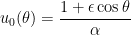
Step 0. Ignore the general-relativity contribution and solve the simpler initial-value problem

$u_0''(\theta) + u_0(\theta) = \displaystyle \frac{1}{\alpha}$

$u_0(0) = \displaystyle \frac{1 + \epsilon}{\alpha}$

$u_0'(0) = 0$ ,

which is a zeroth-order approximation to the real initial-value problem. We found that the solution of this differential equation is

$u_0(\theta) = \displaystyle \frac{1 + \epsilon \cos \theta}{\alpha}$ ,

which is the equation of an ellipse in polar coordinates.

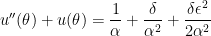
Step 1. Solve the initial-value problem

$u_1''(\theta) + u_1(\theta) = \displaystyle \frac{1}{\alpha} + \delta [u_0(\theta)]^2$

$u_1(0) = \displaystyle \frac{1 + \epsilon}{\alpha}$

$u_1'(0) = 0$ ,

which partially incorporates the term due to general relativity. This is a first-order approximation to the real differential equation. After much effort, we found that the solution of this initial-value problem is

$u_1(\theta) = \displaystyle \frac{1 + \epsilon \cos \theta}{\alpha} + \frac{\delta}{\alpha^2} + \frac{\delta \epsilon^2}{2\alpha^2} + \frac{ \delta\epsilon}{\alpha^2} \theta \sin \theta - \frac{ \delta \epsilon^2}{6\alpha^2} \cos 2\theta - \frac{\delta(3+\epsilon^2)}{3\alpha^2} \cos \theta$ .

For large values of $\theta$ , this is accurately approximated as:

$u_1(\theta) \approx \displaystyle \frac{1 + \epsilon \cos \theta}{\alpha} + \frac{ \delta\epsilon}{\alpha^2} \theta \sin \theta$ ,

which can be further approximated as

$u_1(\theta) \approx \displaystyle \frac{1}{\alpha} \left[ 1 + \epsilon \cos \left( \theta - \frac{\delta \theta}{\alpha} \right) \right]$ .

From this expression, the precession in a planet’s orbit due to general relativity can be calculated.

Roughly 20 years ago, I presented this application of differential equations at the annual meeting of the Texas Section of the Mathematical Association of America. After the talk, a member of the audience asked what would happen if we did this procedure yet again to find a second-order approximation. In other words, I was asked to consider…

Step 2. Solve the initial-value problem

$u_2''(\theta) + u_2(\theta) = \displaystyle \frac{1}{\alpha} + \delta [u_1(\theta)]^2$

$u_2(0) = \displaystyle \frac{1 + \epsilon}{\alpha}$

$u_2'(0) = 0$ .

It stands to reason that the answer should be an even more accurate approximation to the true solution $u(\theta)$ .

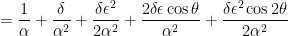
I didn’t have an immediate answer for this question, but I can answer it now. Letting Mathematica do the work, here’s the answer:

Yes, it’s a mess. The term in red is $u_0(\theta)$ , while the term in yellow is the next largest term in $u_1(\theta)$ . Both of these appear in the answer to $u_2(\theta)$ .

The term in green is the next largest term in $u_2(\theta)$ , with the highest power of $\theta$ in the numerator and the highest power of $\alpha$ in the denominator. In other words,

$u_2(\theta) \approx \displaystyle \frac{1 + \epsilon \cos \theta}{\alpha} + \frac{ \delta\epsilon}{\alpha^2} \theta \sin \theta -\frac{\delta^2 \epsilon}{2\alpha^3} \theta^2 \cos \theta$ .

How does this compare to our previous approximation of

$u(\theta) \approx \displaystyle \frac{1}{\alpha} \left[ 1 + \epsilon \cos \left( \theta - \frac{\delta \theta}{\alpha} \right) \right]$ ?

Well, to a second-order Taylor approximation, it’s the same! Let

$f(x) = \displaystyle \frac{1}{\alpha} \left[ 1 + \epsilon \cos \left( \theta - x \right) \right]$ .

Expanding about $x = 0$ and treated $\theta$ as a constant, we find

$f(x) \approx f(0) + f'(0) x + \displaystyle \frac{f''(0)}{2} x^2 = \displaystyle \frac{1}{\alpha} \left[ 1 + \epsilon \cos \left( \theta\right) \right] + \frac{\epsilon}{\alpha} x \sin \theta - \frac{\epsilon}{2\alpha} x^2 \cos \theta$ .

Substituting $x = \displaystyle \frac{\delta \theta}{\alpha}$ yields the above approximation for $u_2(\theta)$ .

Said another way, proceeding to a second-order approximation merely provides additional confirmation for the precession of a planet’s orbit.

Just for the fun of it, I also used Mathematica to find the solution of Step 3:

Step 2. Solve the initial-value problem

$u_3''(\theta) + u_3(\theta) = \displaystyle \frac{1}{\alpha} + \delta [u_2(\theta)]^2$

$u_3(0) = \displaystyle \frac{1 + \epsilon}{\alpha}$

$u_3'(0) = 0$ .

I won’t copy-and-paste the solution from Mathematica; unsurpisingly, it’s really long. I will say that, unsurprisingly, the leading terms are

$u_3(\theta) \approx \displaystyle \frac{1 + \epsilon \cos \theta}{\alpha} + \frac{ \delta\epsilon}{\alpha^2} \theta \sin \theta -\frac{\delta^2 \epsilon}{2 \alpha^3} \theta^2 \cos \theta -\frac{\delta^3 \epsilon}{6\alpha^4} \theta^3 \sin \theta$ .

I said “unsurprisingly” because this matches the third-order Taylor polynomial of our precession expression. I don’t have time to attempt it, but surely there’s a theorem to be proven here based on this computational evidence.

Confirming Einstein’s Theory of General Relativity With Calculus, Part 7e: Computing Precession

We have shown that under general relativity, the motion of a planet around the Sun precesses by

$\phi = \displaystyle \frac{6\pi GM}{ac^2 (1-\epsilon^2)} \qquad \hbox{radians per orbit}$ ,

where $a$ is the semi-major axis of the planet’s orbit, $\epsilon$ is the orbit’s eccentricity, $G$ is the gravitational constant of the universe, $M$ is the mass of the Sun, and $c$ is the speed of light.

Notice that for $\phi$ to be as observable as possible, we’d like $a$ to be as small as possible and $\epsilon$ to be as large as possible. By a fortunate coincidence, the orbit of Mercury — the closest planet to the sun — has the most elliptical orbit of the eight planets.

Here are the values of the constants for Mercury’s orbit in the SI system:

$G = 6.6726 \times 10^{-11} \qquad \hbox{N-m}^2/\hbox{kg}^2$
$M = 1.9929 \times 10^{30} \qquad \hbox{kg}$
$a = 5.7871 \times 10^{10} \qquad \hbox{m}$
$c = 2.9979 \times 10^{8} \qquad \hbox{m/s}$
$\epsilon = 0.2056$
$T = 0.2408 \qquad \hbox{years}$

The last constant, $T$ , is the time for Mercury to complete one orbit. This isn’t in the SI system, but using Earth years as the unit of time will prove useful later in this calculation.

Using these numbers, and recalling that $1 ~ \hbox{N} = 1 ~ \hbox{kg-m/s}^2$ , we find that

$\phi = \displaystyle \frac{6\pi \times 6.6726 \times 10^{-11} ~ \hbox{m}^3/(\hbox{kg-s}^2) \times 1.9929 \times 10^{30} ~ \hbox{kg}}{5.7871 \times 10^{10} ~ \hbox{m} \times (2.9979 \times 10^{8} ~ \hbox{m/s})^2 \times (1-(0.2408)^2)} \approx 5.03 \times 10^{-7}$ .

Notice that all of the units cancel out perfectly; this bit of dimensional analysis is a useful check against careless mistakes.

Again, the units of $\phi$ are in radians per Mercury orbit, or radians per 0.2408 years. We now convert this to arc seconds per century:

$\phi \approx 5.03 \times 10^{-7} \displaystyle \frac{\hbox{radians}}{\hbox{0.2408 years}} \times \frac{180 ~\hbox{degrees}}{\pi ~ \hbox{radians}} \times \frac{3600 ~ \hbox{arc seconds}}{1 ~ \hbox{degree}} \times \frac{100 ~ \hbox{years}}{1 ~ \hbox{century}}$

$\phi = 43.1 \displaystyle \frac{\hbox{arc seconds}}{\hbox{century}}$ .

This indeed matches the observed precession in Mercury’s orbit, thus confirming Einstein’s theory of relativity.

This same computation can be made for other planets. For Venus, we have the new values of $a = 1.0813 \times 10^{11} ~ \hbox{m}$ , $\epsilon = 0.0068$ , and $T = 0.6152 ~ \hbox{years}$ . Repeating this calculation, we predict the precession in Venus’s orbit to be 8.65” per century. Einstein made this prediction in 1915, when the telescopes of the time were not good enough to measure the precession in Venus’s orbit. This only happened in 1960, 45 years later and 5 years after Einstein died. Not surprisingly, the precession in Venus’s orbit also agrees with general relativity.

Confirming Einstein’s Theory of General Relativity With Calculus, Part 7d: Predicting Precession IV

We have shown that the motion of a planet around the Sun, expressed in polar coordinates $(r,theta)$ with the Sun at the origin, under general relativity is

$u(\theta) \approx \displaystyle \frac{1}{\alpha} \left[ 1 + \epsilon \cos \left( \theta - \frac{\delta \theta}{\alpha} \right) \right]$ ,

where $u = \displaystyle \frac{1}{r}$ , $\alpha = a(1-\epsilon^2)$ , $a$ is the semi-major axis of the planet’s orbit, $\epsilon$ is the orbit’s eccentricity, $\delta = \displaystyle \frac{3GM}{c^2}$ , $G$ is the gravitational constant of the universe, $m$ is the mass of the planet, $M$ is the mass of the Sun, $P$ is the planet’s perihelion, $\ell$ is the constant angular momentum of the planet, and $c$ is the speed of light.

The above function $u(\theta)$ is maximized (i.e., the distance from the Sun $r(\theta)$ is minimized) when $\displaystyle \cos \left( \theta - \frac{\delta \theta}{\alpha} \right)$ is as large as possible. This occurs when $\theta - \displaystyle \frac{\delta \theta}{\alpha}$ is a multiple of $2\pi$ .

Said another way, the planet is at its closest point to the Sun when $\theta = 0$ . One orbit later, the planet returns to its closest point to the Sun when

$\theta - \displaystyle \frac{\delta \theta}{\alpha} = 2\pi$

$\theta \displaystyle\left(1 - \frac{\delta}{\alpha} \right) = 2\pi$

$\theta = 2\pi \displaystyle\frac{1}{1 - (\delta/\alpha)}$

We now use the approximation

$\displaystyle \frac{1}{1-x} \approx 1 + x \qquad \hbox{if} \qquad x \approx 0$ ;

this can be demonstrated by linearization, Taylor series, or using the first two terms of the geometric series $1 + x + x^2 + x^3 + \dots$ . With this approximation, the closest approach to the Sun in the next orbit occurs when

$\theta = 2\pi \displaystyle\left(1 + \frac{\delta}{\alpha} \right) = 2\pi + \frac{2\pi \delta}{\alpha}$ ,

which is coterminal with the angle

$\phi = \displaystyle \frac{2\pi \delta}{\alpha}$ .

Substituting $\alpha = a(1-\epsilon^2)$ and $\delta = \displaystyle \frac{3GM}{c^2}$ , we see that the amount of precession per orbit is

$\phi = \displaystyle 2 \pi \frac{3GM}{c^2} \frac{1}{a(1-\epsilon^2)} = \frac{6\pi G M}{ac^2(1-\epsilon^2)}$ .

The units of $\phi$ are radians per orbit. In the next post, we will use Mercury’s data to find $\phi$ in seconds of arc per century.

Confirming Einstein’s Theory of General Relativity With Calculus, Part 7c: Predicting Precession III

We have shown that the motion of a planet around the Sun, expressed in polar coordinates $(r,theta)$ with the Sun at the origin, under general relativity is

$u(\theta) \approx \displaystyle \frac{1}{\alpha} \left[ 1 + \epsilon \cos \left( \theta - \frac{\delta \theta}{\alpha} \right) \right]$ ,

where $u = \displaystyle \frac{1}{r}$ , $\displaystyle \frac{1}{\alpha} = \frac{GMm^2}{\ell^2}$ , $\epsilon = \displaystyle \frac{\alpha - P}{P}$ , $\delta = \displaystyle \frac{3GM}{c^2}$ , $G$ is the gravitational constant of the universe, $m$ is the mass of the planet, $M$ is the mass of the Sun, $P$ is the planet’s perihelion, $\ell$ is the constant angular momentum of the planet, and $c$ is the speed of light.

We notice that the orbit of a planet under general relativity looks very, very similar to the orbit under Newtonian physics:

$u(\theta) \approx \displaystyle \frac{1}{\alpha} \left[ 1 + \epsilon \cos \theta \right]$ ,

so that

$r(\theta) = \displaystyle \frac{\alpha}{1 + \epsilon \cos \theta}$ .

As we’ve seen, this describes an elliptical orbit, normally expressed in rectangular coordinates as

$\displaystyle \frac{(x-h)^2}{a^2} + \frac{y^2}{b^2} = 1$ ,

with semimajor axis along the $x-$ axis. In particular, for an elliptical orbit, the planet’s closest approach to the Sun occurs at $\theta = 0$ :

$r(0) = \displaystyle \frac{\alpha}{1 + \epsilon \cos 0} = \frac{\alpha}{1 + \epsilon}$ ,

and the planet’s further distance from the Sun occurs at $\theta = \pi$ :

$r(\pi) = \displaystyle \frac{\alpha}{1 + \epsilon \cos \pi} = \frac{\alpha}{1 - \epsilon}$ .

Therefore, the length $2a$ of the major axis of the ellipse is the sum of these two distances:

$2a = \displaystyle \frac{\alpha}{1 + \epsilon} + \frac{\alpha}{1 - \epsilon}$

$2a = \displaystyle \frac{\alpha(1-\epsilon) + \alpha(1+\epsilon)}{(1 + \epsilon)(1 - \epsilon)}$

$2a= \displaystyle \frac{2\alpha}{1 - \epsilon^2}$

$a = \displaystyle \frac{\alpha}{1 - \epsilon^2}$ .

Said another way, $\alpha = a(1-\epsilon^2)$ . This is a far more convenient formula for computing $\alpha$ than $\alpha = \displaystyle \frac{\ell^2}{GMm^2}$ , as the values of $a$ (the semi-major axis) and $\epsilon$ (the eccentricity of the orbit) are more accessible than the angular momentum $\ell$ of the planet’s orbit.

In the next post, we finally compute the precession of the orbit.

Confirming Einstein’s Theory of General Relativity With Calculus, Part 7b: Predicting Precession II

We have shown that the motion of a planet around the Sun, expressed in polar coordinates $(r,\theta)$ with the Sun at the origin, under general relativity is

$u(\theta) \approx \displaystyle \frac{1 + \epsilon \cos \theta}{\alpha} + \frac{ \delta\epsilon}{\alpha^2} \theta \sin \theta$ ,

We will now simplify this expression, using the facts that $\delta$ is very small and $\alpha$ is quite large, so that $\delta/\alpha$ is very small indeed. We will use the two approximations

$\cos x \approx 1 \qquad \hbox{and} \qquad \sin x \approx x \qquad \hbox{if} \qquad x \approx 0$ ;

these approximations can be obtained by linearization or else using the first term of the Taylor series expansions of $\cos x$ and $\sin x$ about $x = 0$ .

We will also need the trig identity

$\cos(\theta_1 - \theta_2) = \cos \theta_1 \cos \theta_2 + \sin \theta_1 \sin \theta_2$ .

With these tools, we can now simplify $u(\theta)$ :

$u(\theta) \approx \displaystyle \frac{1 + \epsilon \cos \theta}{\alpha} + \frac{ \delta\epsilon}{\alpha^2} \theta \sin \theta$

$= \displaystyle \frac{1}{\alpha} \left[1 + \epsilon \cos \theta + \frac{ \delta\epsilon}{\alpha} \theta \sin \theta \right]$

$= \displaystyle \frac{1}{\alpha} \left[1 + \epsilon \left(\cos \theta + \frac{ \delta}{\alpha} \theta \sin \theta \right) \right]$

$= \displaystyle \frac{1}{\alpha} \left[1 + \epsilon \left(\cos \theta \cdot 1 + \sin \theta \cdot \frac{ \delta \theta}{\alpha} \right) \right]$

$\approx \displaystyle \frac{1}{\alpha} \left[1 + \epsilon \left(\cos \theta \cdot \cos \frac{\delta \theta}{\alpha} + \sin \theta \cdot \sin \frac{ \delta \theta}{\alpha} \right) \right]$

$\approx \displaystyle \frac{1}{\alpha} \left[1 + \epsilon \cos \left( \theta - \frac{\delta \theta}{\alpha} \right) \right]$ .

Confirming Einstein’s Theory of General Relativity With Calculus, Part 7a: Predicting Precession I

We have shown that the motion of a planet around the Sun, expressed in polar coordinates $(r,\theta)$ with the Sun at the origin, under general relativity is

$u(\theta) = \displaystyle \frac{1 + \epsilon \cos \theta}{\alpha} + \frac{\delta}{\alpha^2} + \frac{\delta \epsilon^2}{2\alpha^2} + \frac{ \delta\epsilon}{\alpha^2} \theta \sin \theta - \frac{ \delta \epsilon^2}{6\alpha^2} \cos 2\theta - \frac{\delta(3+\epsilon^2)}{3\alpha^2} \cos \theta$ ,

We notice that the first term of the above solution,

$\displaystyle \frac{1 + \epsilon \cos \theta}{\alpha}$ ,

is the same as the solution found earlier under Newtonian physics, without general relativity. Therefore, the remaining terms describe the perturbation due to general relativity. All of these terms contain the small factor $\delta$ , and so these can be expected to be small adjustments to an elliptical orbit.

Of these terms, the terms

$\displaystyle \frac{\delta}{\alpha^2} + \frac{\delta \epsilon^2}{2\alpha^2}$

are constants, while the terms

$- \displaystyle \frac{ \delta \epsilon^2}{6\alpha^2} \cos 2\theta - \frac{\delta(3+\epsilon^2)}{3\alpha^2} \cos \theta$

is bounded since $-1 \le \cos \theta \le 1$ and $-1 \le \cos 2\theta \le 1$ . By contrast, the term

$\displaystyle \frac{ \delta\epsilon}{\alpha^2} \theta \sin \theta$

grows without bound. Therefore, for large values of $\theta$ , the planet’s orbit may be accurately described by only including this last perturbation:

$u(\theta) = \displaystyle \frac{1 + \epsilon \cos \theta}{\alpha} + \frac{ \delta\epsilon}{\alpha^2} \theta \sin \theta$ .

In the next post, we simplify this even further.

Confirming Einstein’s Theory of General Relativity With Calculus, Part 6k: Solving New Differential Equation with Method of Undetermined Coefficients

We have shown that the motion of a planet around the Sun, expressed in polar coordinates $(r,\theta)$ with the Sun at the origin, under general relativity follows the initial-value problem

$u''(\theta) + u(\theta) = \displaystyle \frac{1}{\alpha} + \frac{\delta}{\alpha^2} + \frac{\delta \epsilon^2}{2\alpha^2} + \frac{2\delta \epsilon \cos \theta}{\alpha^2} + \frac{\delta \epsilon^2 \cos 2\theta}{2\alpha^2}$ ,

$u(0) = \displaystyle \frac{1}{P}$ ,

$u'(0) = 0$ ,

where $u = \displaystyle \frac{1}{r}$ , $\displaystyle \frac{1}{\alpha} = \frac{GMm^2}{\ell^2}$ , $\delta = \displaystyle \frac{3GM}{c^2}$ , $G$ is the gravitational constant of the universe, $m$ is the mass of the planet, $M$ is the mass of the Sun, $\ell$ is the constant angular momentum of the planet, $c$ is the speed of light, and $P$ is the smallest distance of the planet from the Sun during its orbit (i.e., at perihelion).

In recent posts, we used the method of undetermined coefficients to show that the general solution of the differential equation is

$u(\theta) = c_1 \cos \theta + c_2 \sin \theta + \displaystyle \frac{1}{\alpha} + \frac{\delta}{\alpha^2} + \frac{\delta \epsilon^2}{2\alpha^2} +\frac{\delta \epsilon}{\alpha^2} \theta \sin \theta- \frac{\delta \epsilon^2}{6\alpha^2} \cos 2\theta$ .

We now use the initial conditions to find the constants $c_1$ and $c_2$ . (We did this earlier when we solved the differential equation via variation of parameters, but we repeat the argument here for completeness.) From the initial condition $u(0) = \displaystyle \frac{1}{P} = \frac{1+\epsilon}{\alpha}$ , we obtain

$u(0) = \displaystyle c_1 \cos 0 + c_2 \sin 0 + \displaystyle \frac{1}{\alpha} + \frac{\delta}{\alpha^2} + \frac{\delta \epsilon^2}{2\alpha^2} + \frac{\delta \epsilon \cdot 0 \cdot \sin 0}{\alpha^2} -\frac{\delta \epsilon^2 \cos 0}{6\alpha^2}$

$\displaystyle \frac{1+\epsilon}{\alpha} = c_1 + \displaystyle \frac{1}{\alpha} + \frac{\delta}{\alpha^2} + \frac{\delta \epsilon^2}{2\alpha^2} -\frac{\delta \epsilon^2}{6\alpha^2}$

$\displaystyle \frac{\epsilon}{\alpha} = c_1 + \displaystyle \frac{3\delta +\delta \epsilon^2}{3\alpha^2}$ ,

so that

$c_1 = \displaystyle \frac{\epsilon}{\alpha} - \frac{\delta(3 + \epsilon^2)}{3\alpha^2}$ .

Next, we compute $u'(\theta)$ and use the initial condition $u'(0) = 0$ :

$u'(\theta) = \displaystyle -c_1 \sin \theta + c_2 \cos \theta + \frac{\delta \epsilon}{\alpha^2} (\sin \theta + \theta \cos \theta) + \frac{\delta \epsilon^2 \sin 2\theta}{3\alpha^2}$

$u'(0) = \displaystyle -c_1 \sin 0 + c_2 \cos 0 + \frac{\delta \epsilon}{\alpha^2} (\sin 0 + 0 \cos 0) + \frac{\delta \epsilon^2 \sin 0}{3\alpha^2}$

$0 = c_2$ .

Substituting these values for $c_1$ and $c_2$ , we finally arrive at the solution

$u(\theta) = \displaystyle \left(\frac{\epsilon}{\alpha} - \frac{\delta(3 + \epsilon^2)}{3\alpha^2} \right) \cos \theta + \displaystyle \frac{1}{\alpha} + \frac{\delta}{\alpha^2} + \frac{\delta \epsilon^2}{2\alpha^2} + \frac{\delta \epsilon \theta \sin \theta}{\alpha^2} -\frac{\delta \epsilon^2 \cos 2\theta}{6\alpha^2}$

$= \displaystyle \frac{1 + \epsilon \cos \theta}{\alpha} + \frac{\delta}{\alpha^2} + \frac{\delta \epsilon^2}{2\alpha^2} + \frac{ \delta\epsilon}{\alpha^2} \theta \sin \theta - \frac{ \delta \epsilon^2}{6\alpha^2} \cos 2\theta - \frac{\delta(3+\epsilon^2)}{3\alpha^2} \cos \theta$ .

Confirming Einstein’s Theory of General Relativity With Calculus, Part 6j: Rationale for Method of Undetermined Coefficients VII

We have shown that the motion of a planet around the Sun, expressed in polar coordinates $(r,\theta)$ with the Sun at the origin, under general relativity follows the initial-value problem

$u(0) = \displaystyle \frac{1}{P}$ ,

$u'(0) = 0$ ,

where $u = \displaystyle \frac{1}{r}$ , $\displaystyle \frac{1}{\alpha} = \frac{GMm^2}{\ell^2}$ , $\delta = \displaystyle \frac{3GM}{c^2}$ , $G$ is the gravitational constant of the universe, $m$ is the mass of the planet, $M$ is the mass of the Sun, $\ell$ is the constant angular momentum of the planet, $c$ is the speed of light, and $P$ is the smallest distance of the planet from the Sun during its orbit (i.e., at perihelion).

Let me summarize the partial results that we’ve found in the past few posts.

1. The general solution of the associated homogeneous differential equation

$u''(\theta) + u(\theta) = 0$

$u_0(\theta) = c_1 \cos \theta + c_2 \sin \theta$ .

2. One particular solution of the nonhomogeneous differentiatial equation

$u''(\theta) + u(\theta) = \displaystyle \frac{1}{\alpha} + \frac{\delta}{\alpha^2} + \frac{\delta \epsilon^2}{2\alpha^2}$

$u_1(\theta) = \displaystyle \frac{1}{\alpha} + \frac{\delta}{\alpha^2} + \frac{\delta \epsilon^2}{2\alpha^2}$ .

3. One particular solution of the nonhomogeneous differential equation

$u''(\theta) + u(\theta) = \displaystyle \frac{2\delta \epsilon \cos \theta}{\alpha^2}$

$u_2(\theta) = \displaystyle \frac{\delta \epsilon}{\alpha^2} \theta \sin \theta$ .

4. One particular solution of the nonhomogeneous differential equatio

$u''(\theta) + u(\theta) = \displaystyle \frac{\delta \epsilon^2 \cos 2\theta}{2\alpha^2}$

$u_3(\theta) = \displaystyle -\frac{\delta \epsilon^2}{6\alpha^2} \cos 2\theta$ .

To solve the original differential equation, we will simply add these four solutions together:

$u(\theta) = u_0(\theta) + u_1(\theta) + u_2(\theta) + u_3(\theta)$

$= c_1 \cos \theta + c_2 \sin \theta + \displaystyle \frac{1}{\alpha} + \frac{\delta}{\alpha^2} + \frac{\delta \epsilon^2}{2\alpha^2} +\frac{\delta \epsilon}{\alpha^2} \theta \sin \theta- \frac{\delta \epsilon^2}{6\alpha^2} \cos 2\theta$ .

It’s a straightforward exercise to show that this new function satisfies the original differential equation:

$u''(\theta) + u(\theta) = u_0''(\theta) + u_1''(\theta) + u_2''(\theta) + u_3''(\theta) + u_0(\theta) + u_1(\theta) + u_2(\theta) + u_3(\theta)$

$= [u_0''(\theta) +u_0(\theta)]+ [u_1''(\theta) + u_1(\theta)]+[u_2''(\theta) + u_2(\theta)] + [u_3''(\theta) + u_3(\theta)]$

$= 0 + \displaystyle \left( \frac{1}{\alpha} + \frac{\delta}{\alpha^2} + \frac{\delta \epsilon^2}{2\alpha^2} \right) + \frac{2\delta \epsilon \cos \theta}{\alpha^2} + \frac{\delta \epsilon^2 \cos 2\theta}{2\alpha^2}$

$= \displaystyle \frac{1}{\alpha} + \frac{\delta}{\alpha^2} + \frac{\delta \epsilon^2}{2\alpha^2} + \frac{2\delta \epsilon \cos \theta}{\alpha^2} + \frac{\delta \epsilon^2 \cos 2\theta}{2\alpha^2}$ ,

as required.