Confirming Einstein’s Theory of General Relativity With Calculus, Part 5b: Deriving Orbits under Newtonian Mechanics with Calculus

In this series, I’m discussing how ideas from calculus and precalculus (with a touch of differential equations) can predict the precession in Mercury’s orbit and thus confirm Einstein’s theory of general relativity. The origins of this series came from a class project that I assigned to my Differential Equations students maybe 20 years ago.

We previously showed that if the motion of a planet around the Sun is expressed in polar coordinates $(r,theta)$ , with the Sun at the origin, then under Newtonian mechanics (i.e., without general relativity) the motion of the planet follows the differential equation

$u''(\theta) + u(\theta) = \displaystyle \frac{1}{\alpha}$ ,

where $u = 1/r$ and $\alpha$ is a certain constant. We will also impose the initial condition that the planet is at perihelion (i.e., is closest to the sun), at a distance of $P$ , when $\theta = 0$ . This means that $u$ obtains its maximum value of $1/P$ when $\theta = 0$ . This leads to the two initial conditions

$u(0) = \displaystyle \frac{1}{P} \qquad \hbox{and} \qquad u'(0) = 0$ ;

the second equation arises since $u$ has a local extremum at $\theta = 0$ .

In the previous post, we confirmed that

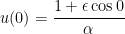
$u(\theta) = \displaystyle \frac{1 + \epsilon \cos \theta}{\alpha}$

solved this initial-value problem. However, the solution was unsatisfying because it gave no indication of where this guess might have come from. In this post, I suggest a series of questions that good calculus students could be asked that would hopefully lead them quite naturally to this solution.

Step 1. Let’s make the differential equation simpler, for now, by replacing the right-hand side with 0:

$u''(\theta) + u(\theta) = 0$ ,

or

$u''(\theta) = -u(\theta)$ .

Can you think of a function or two that, when you differentiate twice, you get the original function back, except with a minus sign in front?

Answer to Step 1. With a little thought, hopefully students can come up with the standard answers of $u(\theta) = \cos \theta$ and $u(\theta) = \sin \theta$ .

Step 2. Using these two answers, can you think of a third function that works?

Answer to Step 2. This is usually the step that students struggle with the most, as they usually try to think of something completely different that works. This won’t work, but that’s OK… we all learn from our failures. If they can’t figure out, I’ll give a big hint: “Try multiplying one of these two answers by something.” In time, they’ll see that answers like $u(\theta) = 2\cos \theta$ and $u(\theta) = 3\sin \theta$ work. Once that conceptual barrier is broken, they’ll usually produce the solutions $u(\theta) = a \cos \theta$ and $u(\theta) = b \sin \theta$ .

Step 3. Using these two answers, can you think of anything else that works?

Answer to Step 3. Again, students might struggle as they imagine something else that works. If this goes on for too long, I’ll give a big hint: “Try combining them.” Eventually, we hopefully get to the point that they’ll see that the linear combination $u(\theta) = a \cos \theta + b \sin \theta$ also solves the associated homogeneous differential equation.

Step 4. Let’s now switch back to the original differential equation $u''(\theta) + u(\theta) = \displaystyle \frac{1}{\alpha}$ . Let’s start simple: $u''(\theta) + u(\theta) = 5$ . Can you think of an easy function that’s a solution?

Answer to Step 4. This might take some experimentation, and students will probably try unnecessarily complicated guesses first. If this goes on for too long, I’ll give a big hint: “Try a constant.” Eventually, they hopefully determine that if $u(\theta) = 5$ is a constant function, then clearly $u'(\theta) = 0$ and $u''(\theta) = 0$ , so that $u''(\theta) + u(\theta) = 5$ .

Step 5. Let’s return to $u''(\theta) + u(\theta) = \displaystyle \frac{1}{\alpha}$ . Any guesses on an answer to this one?

Answer to Step 5. Hopefully, students quickly realize that the constant function $u(\theta) = \displaystyle \frac{1}{\alpha}$ works.

Step 6. Let’s review. We’ve shown that anything of the form $u(\theta) = a\cos \theta + b \sin \theta$ is a solution of $u''(\theta) + u(\theta) = 0$ . We’ve also shown that $u(\theta) = \displaystyle\frac{1}{\alpha}$ is a solution of $u''(\theta) + u(\theta) = \displaystyle \frac{1}{\alpha}$ . Can you think use these two answers to find something else that works?

Answer to Step 6. Hopefully, with the experience learned from Step 3, students will guess that $u(\theta) = a\cos \theta + b\sin \theta + \displaystyle \frac{1}{\alpha}$ will work.

Step 7. OK, that solves the differential equation. Any thoughts on how to find the values of $a$ and $b$ so that $u(0) = \displaystyle \frac{1}{P}$ and $u'(0) = 0$ ?

Answer to Step 7. Hopefully, students will see that we should just plug into $u(\theta)$ :

$u(0) = a \cos 0 + b \sin 0 + \displaystyle \frac{1}{\alpha}$

$\displaystyle \frac{1}{P} = a + \frac{1}{\alpha}$

$\displaystyle \frac{1}{P} - \frac{1}{\alpha} = a$

$\displaystyle \frac{\alpha - P}{\alpha P} = a$

To find $b$ , we first find $u'(\theta)$ and then substitute $\theta = 0$ :

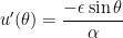
$u'(\theta) = -a \sin \theta + b \cos \theta$

$u'(0) = -a \sin 0 + b \cos 0$

$0 = b$ .

From these two constants, we obtain

$u(\theta) = \displaystyle \frac{\alpha - P}{\alpha P} \cos \theta + 0 \sin \theta + \displaystyle \frac{1}{\alpha}$

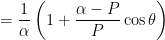
$= \displaystyle \frac{1}{\alpha} \left( 1 + \frac{\alpha-P}{P} \cos \theta \right)$

$= \displaystyle \frac{1 + \epsilon \cos \theta}{\alpha}$ ,

where $\epsilon = \displaystyle \frac{\alpha - P}{P}$ .

Finally, since $r = 1/u$ , we see that the planet’s orbit satisfies

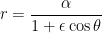
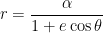
$r = \displaystyle \frac{\alpha}{1 + \epsilon \cos \theta}$ ,

so that, as shown earlier in this series, the orbit is an ellipse with eccentricity $\epsilon$ .

Confirming Einstein’s Theory of General Relativity With Calculus, Part 5a: Confirming Orbits under Newtonian Mechanics with Calculus

We previously showed that if the motion of a planet around the Sun is expressed in polar coordinates $(r,\theta)$ , with the Sun at the origin, then under Newtonian mechanics (i.e., without general relativity) the motion of the planet follows the differential equation

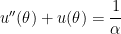
$u''(\theta) + u(\theta) = \displaystyle \frac{1}{\alpha}$ ,

$u(0) = \displaystyle \frac{1}{P} \qquad \hbox{and} \qquad u'(0) = 0$ ;

the second equation arises since $u$ has a local extremum at $\theta = 0$ .

In the next few posts, we’ll discuss the solution of this initial-value problem. Today’s post would be appropriate for calculus students, which is confirming that

$u(\theta) = \displaystyle \frac{1 + \epsilon \cos \theta}{\alpha}$

solves this initial-value problem, where $\epsilon = \displaystyle \frac{\alpha-P}{P}$ . Since $r$ is the reciprocal of $u$ , we infer that

$r = \displaystyle \frac{\alpha}{1 + \epsilon \cos \theta}$ .

As we’ve already seen in this series, this means that the orbit of the planet is a conic section — either a circle, ellipse, parabola, or hyperbola. Since the orbit of a planet is stable and $\epsilon = 0$ is extremely unlikely, this means that the planet orbits the Sun in an ellipse, with the Sun at one focus of the ellipse.

So, for a calculus student to verify that planets move in ellipses, one must check that

$u(\theta) = \displaystyle \frac{1 + \epsilon \cos \theta}{\alpha}$

is a solution of the initial-value problem

$u''(\theta) + u(\theta) = \displaystyle \frac{1}{\alpha}$ ,

$u(0) = \displaystyle \frac{1}{P}$ ,

$u'(0) = 0$ .

The second line is easy to check:

$u(0) = \displaystyle \frac{1 + \epsilon \cos 0}{\alpha}$

$= \displaystyle \frac{1 + \epsilon}{\alpha}$

$= \displaystyle \frac{1 + \displaystyle \frac{\alpha-P}{P}}{\alpha}$

$= \displaystyle \frac{1}{\alpha} \frac{P + \alpha - P}{P}$

$= \displaystyle \frac{1}{\alpha} \frac{\alpha}{P}$

$= \displaystyle \frac{1}{P}$ .

The third line is also easy to check:

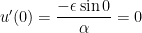
$u'(\theta) = \displaystyle \frac{-\epsilon \sin \theta}{\alpha}$

$u'(0) = \displaystyle \frac{-\epsilon \sin 0}{\alpha} = 0$ .

To check the first line, we first find $u''(\theta)$ :

$u''(\theta) = \displaystyle \frac{-\epsilon \cos \theta}{\alpha}$ ,

so that

$u''(\theta) + u(\theta) = \displaystyle \frac{-\epsilon \cos \theta}{\alpha} + \frac{1 + \epsilon \cos \theta}{\alpha} = \frac{1}{\alpha}$ ,

thus confirming that $u(\theta) = \displaystyle \frac{1 + \epsilon \cos \theta}{\alpha}$ solves the initial-value problem.

While the above calculations are well within the grasp of a good Calculus I student, I’ll be the first to admit that this solution is less than satisfying. We just mysteriously proposed a solution, seemingly out of thin air, and confirmed that it worked. In the next post, I’ll proposed a way that calculus students can be led to guess this solution. Then, we talk about finding the solution of this nonhomogeneous initial-value problem using standard techniques from differential equations.

Confirming Einstein’s Theory of General Relativity With Calculus, Part 4c: Newton’s Second Law and Newton’s Law of Gravitation

In this post, following from the previous two posts, we will show that if the motion of a planet around the Sun is expressed in polar coordinates $(r,\theta)$ , with the Sun at the origin, then under Newtonian mechanics (i.e., without general relativity) the motion of the planet follows the differential equation

$u''(\theta) + u(\theta) = \displaystyle \frac{1}{\alpha}$ ,

where $u = 1/r$ and $\alpha$ is a certain constant. Deriving this governing differential equation will require some principles from physics. If you’d rather skip the physics and get to the mathematics, we’ll get to solving this differential equations in the next post.

From Newton’s second law, the gravitational force on the planet as it orbits the Sun satisfies

${\bf F} = m{\bf a}$ ,

where the force ${\bf F}$ and the acceleration ${\bf a}$ are vectors. When written in polar coordinates, this becomes

${\bf F} = m \displaystyle \left[ \frac{d^2r}{dt^2} - r \left( \frac{d\theta}{dt} \right)^2 \right] {\bf u}_r + m \left(r \frac{d^2 \theta}{d t^2} + 2 \frac{dr}{dt} \frac{d\theta}{dt} \right) {\bf u}_\theta$ ,

where ${\bf u}_r$ is a unit vector pointing away from the origin and ${\bf u}_\theta$ is a unit vector perpendicular to ${\bf u}_r$ that points in the direction of increasing $\theta$ .

Furthermore, from Newton’s Law of Gravitation, if the Sun is located at the origin, then the gravitational force on the planet is

${\bf F} = \displaystyle -\frac{GMm}{r^2} {\bf u}_r$ ,

where $M$ is the mass of the sun, $m$ is the mass of the planet, and $G$ is the gravitational constant of the universe (which is a constant, no matter what Q from Star Trek: The Next Generation says).

Since these are the same force, the ${\bf u}_r$ components must be the same. (Also, the ${\bf u}_\theta$ component must be zero, but we won’t need to use that fact.) Therefore,

$m \displaystyle \left[ \frac{d^2r}{dt^2} - r \left( \frac{d\theta}{dt} \right)^2 \right] = \displaystyle -\frac{GMm}{r^2}$ ,

$\displaystyle \frac{d^2r}{dt^2} - r \left( \frac{d\theta}{dt} \right)^2 = \displaystyle -\frac{GM}{r^2}$ .

In a previous post, we showed that

$\displaystyle \frac{d\theta}{dt} = \frac{\ell}{mr^2}$ ,

where $\ell$ is a constant, and

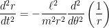
$\displaystyle \frac{d^2r}{dt^2} = - \frac{\ell^2}{m^2 r^2} \frac{d^2}{d\theta^2} \left( \frac{1}{r} \right)$ .

Substituting, we find

$\displaystyle - \frac{\ell^2}{m^2 r^2} \frac{d^2}{d\theta^2} \left( \frac{1}{r} \right) - r \left( \frac{\ell}{mr^2} \right)^2 = \displaystyle -\frac{GM}{r^2}$

$\displaystyle \frac{\ell^2}{m^2 r^2} \frac{d^2}{d\theta^2} \left( \frac{1}{r} \right) + r \left( \frac{\ell^2}{m^2 r^4} \right) = \displaystyle \frac{GM}{r^2}$

$\displaystyle \frac{\ell^2}{m^2 r^2} \frac{d^2}{d\theta^2} \left( \frac{1}{r} \right) +\frac{\ell^2}{m^2 r^3} = \displaystyle \frac{GM}{r^2}$

$\displaystyle \frac{\ell^2}{m^2 r^2} \left[ \frac{d^2}{d\theta^2} \left( \frac{1}{r} \right) + \frac{1}{r} \right] = \displaystyle \frac{GM}{r^2}$

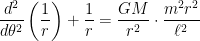
$\displaystyle \frac{d^2}{d\theta^2} \left( \frac{1}{r} \right) + \frac{1}{r} = \displaystyle \frac{GM}{r^2} \cdot \frac{m^2 r^2}{\ell^2}$

$\displaystyle \frac{d^2}{d\theta^2} \left( \frac{1}{r} \right) + \frac{1}{r} = \displaystyle \frac{GMm^2}{\ell^2}$ .

So, substituting $u = 1/r$ and $\alpha = \displaystyle \frac{\ell^2}{GMm^2}$ , we finally obtain the governing equation

$\displaystyle \frac{d^2 u}{d\theta^2} + u = \displaystyle \frac{1}{\alpha}$ .

This is the governing differential equation of planetary motion under Newtonian mechanics. For now, it’s not obvious why we chose $\displaystyle \frac{1}{\alpha}$ as the constant on the right-hand side instead of just $\alpha$ , but the reason for this choice will become apparent in future posts.

In the next few posts, we use differential equations (or, if you’d prefer, just calculus) to show that Newtonian mechanics predicts that planets orbit the Sun in ellipses.

Confirming Einstein’s Theory of General Relativity With Calculus, Part 4b: Acceleration in Polar Coordinates

In this part of the series, we will show that if the motion of a planet around the Sun is expressed in polar coordinates $(r,\theta)$ , with the Sun at the origin, then under Newtonian mechanics (i.e., without general relativity) the motion of the planet follows the differential equation

$u''(\theta) + u(\theta) = \displaystyle \frac{1}{\alpha}$ ,

Part of the derivation of this governing differential equation will involve Newton’s Second Law

${\bf F} = m {\bf a}$ ,

where $m$ is the mass of the planet and the force ${\bf F}$ and the acceleration $a$ are vectors. In usual rectangular coordinates, the acceleration vector would be expressed as

${\bf a} = x''(t) {\bf i} + y''(t) {\bf j}$ ,

where the components of the acceleration in the $x-$ and $y-$ directors are $x''(t)$ and $y''(t)$ , and the unit vectors ${\bf i}$ and ${\bf j}$ are perpendicular, pointing in the positive $x$ and positive $y$ directions.

Unfortunately, our problem involves polar coordinates, and rewriting the acceleration vector in polar coordinates, instead of rectangular coordinates, is going to take some work.

Suppose that the position of the planet is $(r,\theta)$ in polar coordinates, so that the position in rectangular coordinates is ${\bf r} = (r\cos \theta, r \sin \theta)$ . This may be rewritten as

${\bf r} = r \cos \theta {\bf i} + r \sin \theta {\bf j} = r ( \cos \theta {\bf i} + \sin \theta {\bf j}) = r {\bf u}_r$ ,

where

${\bf u}_r = \cos \theta {\bf i} + \sin \theta {\bf j}$

is a unit vector that points away from the origin. We see that this is a unit vector since

$\parallel {\bf u}_r \parallel = {\bf u}_r \cdot {\bf u}_r = \cos^2 \theta + \sin^2 \theta =1$ .

We also define

${\bf u}_\theta = -\sin \theta {\bf i} + \cos \theta {\bf j}$

to be a unit vector that is perpendicular to ${\bf u}_r$ ; it turns out that ${\bf u}_\theta$ points in the direction of increasing $\theta$ . To see that ${\bf u}_r$ and ${\bf u}_\theta$ are perpendicular, we observe

${\bf u}_r \cdot {\bf u}_\theta = -\sin \theta \cos \theta + \sin \theta \cos \theta = 0$ .

Computing the velocity and acceleration vectors in polar coordinates will have a twist that’s not experienced with rectangular coordinates since both ${\bf u}_r$ and ${\bf u}_\theta$ are functions of $\theta$ . Indeed, we have

$\displaystyle \frac{d{\bf u}_r}{d\theta} = \frac{d \cos \theta}{d\theta} {\bf i} + \frac{d\sin \theta}{d\theta} {\bf j} = -\sin \theta {\bf i} + \cos \theta {\bf j} = {\bf u}_\theta$ .

Furthermore,

$\displaystyle \frac{d{\bf u}_\theta}{d\theta} = -\frac{d \sin \theta}{d\theta} {\bf i} + \frac{d\cos \theta}{d\theta} {\bf j} = -\cos \theta {\bf i} - \sin \theta {\bf j} = -{\bf u}_r$ .

These two equations will be needed in the derivation below.

We are now in position to express the velocity and acceleration of the orbiting planet in polar coordinates. Clearly, the position of the planet is $r {\bf u}_r$ , or a distance $r$ from the origin in the direction of ${\bf u}_r$ . Therefore, by the Product Rule, the velocity of the planet is

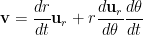
${\bf v} = \displaystyle \frac{d}{dt} (r {\bf u}_r) = \displaystyle \frac{dr}{dt} {\bf u}_r + r \frac{d {\bf u}_r}{dt}$

We now apply the Chain Rule to the second term:

${\bf v} = \displaystyle \frac{dr}{dt} {\bf u}_r + r \frac{d {\bf u}_r}{d\theta} \frac{d\theta}{dt}$

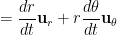
$= \displaystyle \frac{dr}{dt} {\bf u}_r + r \frac{d\theta}{dt} {\bf u}_\theta$ .

Differentiating a second time with respect to time, and again using the Chain Rule, we find

${\bf a} = \displaystyle \frac{d {\bf v}}{dt} = \displaystyle \frac{d^2r}{dt^2} {\bf u}_r + \frac{dr}{dt} \frac{d{\bf u}_r}{dt} + \frac{dr}{dt} \frac{d\theta}{dt} {\bf u}_\theta + r \frac{d^2\theta}{dt^2} {\bf u}_\theta + r \frac{d\theta}{dt} \frac{d{\bf u}_\theta}{dt}$

$= \displaystyle \frac{d^2r}{dt^2} {\bf u}_r + \frac{dr}{dt} \frac{d{\bf u}_r}{d\theta} \frac{d\theta}{dt} + \frac{dr}{dt} \frac{d\theta}{dt} {\bf u}_\theta + r \frac{d^2\theta}{dt^2} {\bf u}_\theta + r \frac{d\theta}{dt} \frac{d{\bf u}_\theta}{d\theta} \frac{d\theta}{dt}$

$= \displaystyle \frac{d^2r}{dt^2} {\bf u}_r + \frac{dr}{dt} \frac{d\theta}{dt} {\bf u}_\theta + \frac{dr}{dt} \frac{d\theta}{dt} {\bf u}_\theta + r \frac{d^2\theta}{dt^2} {\bf u}_\theta - r \left(\frac{d\theta}{dt} \right)^2 {\bf u}_r$

$= \displaystyle \left[ \frac{d^2r}{dt^2} - r \left(\frac{d\theta}{dt} \right)^2 \right] {\bf u}_r + \left[ 2\frac{dr}{dt} \frac{d\theta}{dt} + r \frac{d^2\theta}{dt^2} \right] {\bf u}_\theta$ .

This will be needed in the next post, when we use both Newton’s Second Law and Newton’s Law of Gravitation, expressed in polar coordinates.

Confirming Einstein’s Theory of General Relativity With Calculus, Part 4a: Angular Momentum

$u''(\theta) + u(\theta) = \displaystyle \frac{1}{\alpha}$ ,

One principle from physics that we’ll need is the Law of Conservation of Angular Momentum. Mathematically, this is expressed by

$mr^2 \displaystyle \frac{d\theta}{dt} = \ell$ ,

where $\ell$ is a constant. Of course, this can be written as

$\displaystyle \frac{d\theta}{dt} = \displaystyle \frac{\ell}{mr^2}$ ;

this will be used a couple times in the derivation below.

As we’ll soon see, we will need to express the second derivative $\displaystyle \frac{d^2 r}{d t^2}$ in a form that depends only on $\theta$ . To do this, we use the Chain Rule to obtain

$r' = \displaystyle \frac{dr}{dt}$

$= \displaystyle \frac{dr}{d\theta} \cdot \frac{d\theta}{dt}$

$= \displaystyle \frac{\ell}{mr^2} \frac{dr}{d\theta}$

$= \displaystyle - \frac{\ell}{m} \frac{d}{d\theta} \left( \frac{1}{r} \right)$ .

This last step used the Chain Rule in reverse:

$\displaystyle \frac{d}{d\theta} \left( \frac{1}{r} \right) = \frac{d}{dr} \left( \frac{1}{r} \right) \cdot \frac{dr}{dt} = -\frac{1}{r^2} \cdot \frac{dr}{dt}$ .

To examine the second derivative $\displaystyle \frac{d^2 r}{d t^2}$ , we again use the Chain Rule:

$\displaystyle \frac{d^2 r}{d t^2} = \displaystyle \frac{dr'}{dt}$

$= \displaystyle \frac{dr'}{d\theta} \cdot \frac{d\theta}{dt}$

$= \displaystyle \frac{\ell}{mr^2} \frac{dr'}{d\theta}$

$= \displaystyle \frac{\ell}{mr^2} \frac{d}{d\theta} \left[ \frac{dr}{dt} \right]$

$= \displaystyle \frac{\ell}{mr^2} \frac{d}{d\theta} \left[ - \frac{\ell}{m} \frac{d}{d\theta} \left( \frac{1}{r} \right) \right]$

$= \displaystyle - \frac{\ell^2}{m^2r^2} \frac{d}{d\theta} \left[ \frac{d}{d\theta} \left( \frac{1}{r} \right) \right]$

$= \displaystyle - \frac{\ell^2}{m^2r^2} \frac{d^2}{d\theta^2} \left( \frac{1}{r} \right)$ .

While far from obvious now, this will be needed when we rewrite Newton’s Second Law in polar coordinates.

Confirming Einstein’s Theory of General Relativity With Calculus, Part 3: Method of Successive Approximations

One technique that will be necessary for this confirmation is the method of successive approximations. This will be needed in the context of a differential equation; however, we can illustrate the concept by finding the roots of a polynomial. Consider the quadratic equation

$x^2 - x - 1 = 0$ .

(Naturally, we can solve for $x$ using the quadratic formula; more on that later.) To apply the method of successive approximation, we will rewrite this so that $x$ appears on the left side and some function of $x$ appears on the right side. I will choose

$x^2 = x + 1$ , or

$x = 1 + \displaystyle \frac{1}{x}$ .

Here’s the idea of the method of successive approximations to obtain a recursively defined sequence that (hopefully) convergence to a solution of this equation:

Start with an initial guess $x_0$ .
Plug $x_0$ into the right-hand side to get a new guess, $x_1$ .
Plug $x_1$ into the right-hand side to get a new guess, $x_2$ .
And repeat.

For example, suppose that we choose $x_0 = 1$ . Then

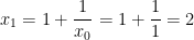
$x_1 = 1 + \displaystyle \frac{1}{x_0} = 1 + \displaystyle \frac{1}{1} = 2$

$x_2 = 1 + \displaystyle \frac{1}{x_1} = 1 + \displaystyle \frac{1}{2} = \displaystyle \frac{3}{2} = 1.5$

$x_3 = 1 + \displaystyle \frac{1}{x_2} = 1 + \displaystyle \frac{1}{3/2} = \displaystyle \frac{5}{3} \approx 1.667$

$x_4 = 1 + \displaystyle \frac{1}{x_3} = 1 + \displaystyle \frac{1}{5/3} = \displaystyle \frac{8}{5} = 1.6$

$x_5 = 1 + \displaystyle \frac{1}{x_4} = 1 + \displaystyle \frac{1}{8/5} = \displaystyle \frac{13}{8} = 1.625$

$x_6 = 1 + \displaystyle \frac{1}{x_5} = 1 + \displaystyle \frac{1}{13/8} = \displaystyle \frac{21}{13} \approx 1.615$

$x_7 = 1 + \displaystyle \frac{1}{x_6} = 1 + \displaystyle \frac{1}{21/13} = \displaystyle \frac{34}{21} \approx 1.619$

This sequence can be computed by entering $1$ into a calculator, then entering $1 + 1 \div \hbox{Ans}$ , and then repeatedly hitting the $=$ button.

We see that the sequence appears to be converging to something, and that something is a root of the equation $x^2 - x - 1 = 0$ , which we now find via the quadratic formula:

$x = \displaystyle \frac{1 \pm \sqrt{1 - 4 \cdot 1 \cdot (-1)}}{2} = \frac{1 \pm \sqrt{5}}{2}$ .

So it looks like the above sequence is converging to the positive root $(1 + \sqrt{5})/2 \approx 1.618$ .

(Parenthetically, you might notice that the Fibonacci sequence appears in the numerators and denominators of this sequence. As you might guess, that’s not a coincidence.)

Like most numerical techniques, this method doesn’t always work like we think it would. Another solution is the negative root $(1 - \sqrt{5})/2 \approx -0.618$ . Unfortunately, if we start with a guess near this root, like $x_0 = -0.62$ , the sequence unexpectedly diverges from $-0.618\dots$ but eventually converges to the positive root $1.618\dots$ :

$x_1 = 1 + \displaystyle \frac{1}{x_0} = 1 + \displaystyle \frac{1}{-0.62} = -0.6129\dots$

$x_2 = 1 + \displaystyle \frac{1}{x_1} = 1 + \displaystyle \frac{1}{-0.6129\dots} = -0.6315\dots$

$x_3 = 1 + \displaystyle \frac{1}{x_2} = 1 + \displaystyle \frac{1}{-0.6315\dots} = -0.5833\dots$

$x_4 = 1 + \displaystyle \frac{1}{x_3} = 1 + \displaystyle \frac{1}{-0.5833\dots} = -0.7142\dots$

$x_5 = 1 + \displaystyle \frac{1}{x_4} = 1 + \displaystyle \frac{1}{-0.5833\dots} = -0.4$

$x_6 = 1 + \displaystyle \frac{1}{x_5} = 1 + \displaystyle \frac{1}{-0.4\dots} = -1.5$

$x_7 = 1 + \displaystyle \frac{1}{x_6} = 1 + \displaystyle \frac{1}{-1.5\dots} = 0.3333\dots$

$x_8 = 1 + \displaystyle \frac{1}{x_7} = 1 + \displaystyle \frac{1}{0.3333\dots} = 4$

$x_9 = 1 + \displaystyle \frac{1}{x_8} = 1 + \displaystyle \frac{1}{4} = 1.25$

$x_{10} = 1 + \displaystyle \frac{1}{x_9} = 1 + \displaystyle \frac{1}{1.25} = 1.8$

$x_{11} = 1 + \displaystyle \frac{1}{x_{10}} = 1 + \displaystyle \frac{1}{1.8} = 1.555\dots$

$x_{12} = 1 + \displaystyle \frac{1}{x_{11}} = 1 + \displaystyle \frac{1}{1.555\dots} = 1.6428\dots$

$x_{13} = 1 + \displaystyle \frac{1}{x_{12}} = 1 + \displaystyle \frac{1}{1.6428\dots} = 1.6086\dots$

$x_{14} = 1 + \displaystyle \frac{1}{x_{13}} = 1 + \displaystyle \frac{1}{1.6086\dots} = 1.6216\dots$

$x_{15} = 1 + \displaystyle \frac{1}{x_{14}} = 1 + \displaystyle \frac{1}{1.6216\dots} = 1.6166\dots$

$x_{16} = 1 + \displaystyle \frac{1}{x_{15}} = 1 + \displaystyle \frac{1}{1.6216\dots} = 1.6185\dots$

I should note that the method of successive approximations generally converges at a slower pace than Newton’s method. However, this method will be good enough when we use it to predict the precession in Mercury’s orbit.

Confirming Einstein’s Theory of General Relativity With Calculus, Part 2d: Hyperbolas and Polar Coordinates

In a previous post, we showed that the polar equation

$r = \displaystyle \frac{a}{1 + e \cos \theta}$

is equivalent to the rectangular equation

$\displaystyle \frac{\left(x + \displaystyle \frac{\alpha e}{1-e^2} \right)^2}{\displaystyle \frac{\alpha^2}{(1-e^2)^2}} + \frac{y^2}{\displaystyle \frac{\alpha^2}{1-e^2}} = 1$

as long as $e \ne 0$ . Furthermore, if $0 < e < 1$ , then this represents an ellipse with eccentricity $e$ whose major axis lies on the $x-$ axis, with one focus located at the origin.

While not directly related to our discussion of precession, it turns out that this equation represents a hyperbola if $e > 1$ . Under this assumption, $1-e^2 < 0$ and $e^2-1>0$ , so let me rewrite the previous equation in terms of $e^2-1$ :

$\displaystyle \frac{\left(x - \displaystyle \frac{\alpha e}{e^2-1} \right)^2}{\displaystyle \frac{\alpha^2}{(e^2-1)^2}} - \frac{y^2}{\displaystyle \frac{\alpha^2}{e^2-1}} = 1$

This matches the form of a left-right hyperbola

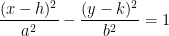
$\displaystyle \frac{(x-h)^2}{a^2} - \frac{(y-k)^2}{b^2} = 1$ ,

where the center of the hyperbola is located at

$(h,k) = \displaystyle \left( \frac{\alpha e}{e^2-1} , 0 \right)$

Also, for a hyperbola, the distance $c$ from the center to the foci satisfies

$c^2 = a^2 + b^2$ ,

so that

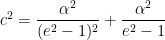
$c^2 = \displaystyle \frac{\alpha^2}{(e^2-1)^2} + \displaystyle \frac{\alpha^2}{e^2-1}$

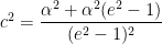
$c^2 = \displaystyle \frac{\alpha^2 + \alpha^2 (e^2 - 1)}{(e^2-1)^2}$

$c^2 = \displaystyle \frac{\alpha^2 e^2}{(e^2-1)^2}$

$c = \displaystyle \frac{\alpha e}{e^2-1}$

The two foci are located a distance $c$ to the left of the right of the center. Since it happened to happen that $c = h$ , this means that the origin is, once again, one of the foci of the hyperbola.

Furthermore, the eccentricity $c/a$ of the hyperbola is easily computed as

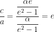
$\displaystyle \frac{c}{a} = \frac{ \displaystyle \frac{\alpha e}{e^2-1} }{ \displaystyle \frac{\alpha}{e^2-1}} = e$ ,

so that, once again, the well-chosen parameter $e$ is the eccentricity.

Confirming Einstein’s Theory of General Relativity With Calculus, Part 2c: Circles, Parabolas, and Polar Coordinates

In the previous post, we showed that the polar equation

$r = \displaystyle \frac{\alpha}{1 + e \cos \theta}$

converts to

$x^2 (1-e^2) + 2 \alpha e x + y^2 = \alpha^2$

in rectangular coordinates. Furthermore, if $0 < e < 1$ , then this represents an ellipse with eccentricity $e$ whose semi-major axis lies along the $x-$ axis with one focus at the origin.

It turns out that, for different non-negative values of $e$ , the same polar equation represents different conic sections. These are not particularly relevant for our study of precession, but I’m including this anyway in this series as a small tangential discussion.

Let’s take a look at the easy case of $e = 0$ . With this substitution, the equation in rectangular coordinates simplifies to

$x^2 + y^2 = \alpha^2$ .

Of course, this is the equation of a circle that is centered at the origin with radius $\alpha$ .

The other easy case is $e = 1$ , so that $1-e^2 = 0$ . Then the equation in rectangular coordinates simplifies to

$2 \alpha x + y^2 = \alpha^2$

$y^2 = -2\alpha x + \alpha^2$

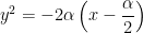
$y^2 = -2 \alpha \displaystyle \left( x - \frac{\alpha}{2} \right)$

$y^2 = -4 \cdot \displaystyle \frac{\alpha}{2} \left( x - \frac{\alpha}{2} \right)$

This matches the form of a parabola that opens to the left with a horizontal axis of symmetry:

$(y-k)^2 = -4 p (x-h)$ .

In this case, the vertex of the parabola is located at

$(h,k) = \displaystyle \left( \frac{\alpha}{2} , 0 \right)$ ,

while the focus of the parabola is located a distance $p = \displaystyle \frac{\alpha}{2}$ to the left of the vertex. In other words, the origin is the focus of the parabola. (For what it’s worth, the directrix of the parabola would be the vertical line $y = \alpha$ , located $p$ to the right of the vertex.)

Confirming Einstein’s Theory of General Relativity With Calculus, Part 2b: Ellipses and Polar Coordinates

As part of our derivation, we’ll need to use the fact that, in polar coordinates, the graph of

$r = \displaystyle \frac{\alpha}{1 + e \cos \theta}$

turns out to be an ellipse if $0 < e < 1$ , with the origin at one focus.

We now prove this. Clearing the denominator, we obtain

$r + re \cos \theta = \alpha$ .

Switching to rectangular coordinates, this becomes

$\sqrt{x^2 + y^2} + e x = \alpha$

$\sqrt{x^2 + y^2} = \alpha - ex$

$x^2 + y^2 = (\alpha - ex)^2$

$x^2 + y^2 = \alpha^2 - 2\alpha ex + e^2 x^2$

$x^2 (1-e^2) + 2 \alpha e x + y^2 = \alpha^2$

$(1-e^2)\left(x^2 + 2 \displaystyle \frac{\alpha e}{1-e^2} x \right) + y^2 = \alpha^2$

$(1-e^2)\left(x^2 + 2 \displaystyle \frac{\alpha e}{1-e^2} x + \frac{\alpha^2 e^2}{(1-e^2)^2} \right) + y^2 = \alpha^2 + \displaystyle \frac{\alpha^2e^2}{1-e^2}$

$(1-e^2) \left(x + \displaystyle \frac{\alpha e}{1-e^2} \right)^2 + y^2 = \displaystyle \frac{\alpha^2(1-e^2)+\alpha^2 e^2}{1-e^2}$

$(1-e^2) \left(x + \displaystyle \frac{\alpha e}{1-e^2} \right)^2 + y^2 = \displaystyle \frac{\alpha^2}{1-e^2}$

$\displaystyle \frac{(1-e^2)^2}{\alpha^2} \left(x + \displaystyle \frac{\alpha e}{1-e^2} \right)^2 + \frac{1-e^2}{\alpha^2} y^2 = 1$

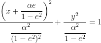
$\displaystyle \frac{\left(x + \displaystyle \frac{\alpha e}{1-e^2} \right)^2}{\displaystyle \frac{\alpha^2}{(1-e^2)^2}} + \frac{y^2}{\displaystyle \frac{\alpha^2}{1-e^2}} = 1$

Since we assumed that $0 < e < 1$ , we have $0 < 1 - e^2 < 1$ so that

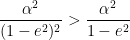
$\displaystyle \frac{\alpha^2}{(1-e^2)^2} > \displaystyle \frac{\alpha^2}{1-e^2}$ .

Therefore, this matches the usual form of an ellipse in rectangular coordinates

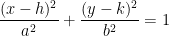
$\displaystyle \frac{(x-h)^2}{a^2} + \frac{(y-k)^2}{b^2} = 1$ ,

where the center of the ellipse is located at

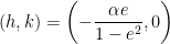
$(h,k) = \displaystyle \left( -\displaystyle \frac{\alpha e}{1-e^2}, 0 \right)$ ,

the semi-major axis is horizontal with length

$a = \displaystyle \frac{\alpha}{1-e^2}$ ,

and the semi-minor axis is vertical with length

$b = \displaystyle \frac{\alpha}{\sqrt{1-e^2}}$ .

Furthermore, the distance $c$ of the foci from the center of the ellipse satisfies the equation

$b^2 + c^2 = a^2$ ,

so that

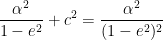
$\displaystyle \frac{\alpha^2}{1-e^2} + c^2 = \displaystyle \frac{\alpha^2}{(1-e^2)^2}$

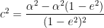
$c^2 = \displaystyle \frac{\alpha^2}{(1-e^2)^2} - \displaystyle \frac{\alpha^2}{1-e^2}$

$c^2 = \displaystyle \frac{\alpha^2 - \alpha^2(1-e^2)}{(1-e^2)^2}$

$c^2 = \displaystyle \frac{\alpha^2 e^2}{(1-e^2)^2}$

$c = \displaystyle \frac{\alpha e}{1-e^2}$

From this, we derive two nice properties of the ellipse. First, looking back on previous work, we see that $c = -h$ . Therefore, since the foci of the ellipse are distance $c$ away from the center along the major axis, we conclude that one focus of the ellipse is located at $(-h+c,0)$ , or $(0,0)$ . That is, the origin is one focus of the ellipse. (For the little it’s worth, the other focus is located at $(-2h,0)$ .

Second, the eccentricity of the ellipse is defined to be the ratio $c/a$ . This is now easily computed:

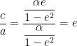
$\displaystyle \frac{c}{a} = \displaystyle \frac{\displaystyle \frac{\alpha e}{1-e^2}}{\displaystyle \frac{\alpha}{1-e^2}} = e$ .

In other words, the letter $e$ was well-chosen to represent the eccentricity of the ellipse.

For what it’s worth, here’s an alternate derivation of the formulas for $a$ and $b$ . For this ellipse, the planet’s closest approach to the Sun occurs at $\theta = 0$ :

$r(0) = \displaystyle \frac{\alpha}{1 + e \cos 0} = \frac{\alpha}{1 + e}$ ,

and the planet’s further distance from the Sun occurs at $\theta = \pi$ :

$r(\pi) = \displaystyle \frac{\alpha}{1 + e \cos \pi} = \frac{\alpha}{1 - e}$ .

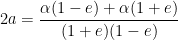
Therefore, the length $2a$ of the major axis of the ellipse is the sum of these two distances:

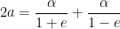
$2a = \displaystyle \frac{\alpha}{1 + e} + \frac{\alpha}{1 - e}$

$2a = \displaystyle \frac{\alpha(1-e) + \alpha(1+e)}{(1 + e)(1 -e)}$

$2a= \displaystyle \frac{2\alpha}{1 - e^2}$

$a = \displaystyle \frac{\alpha}{1 - e^2}$ .

Since $c = a\epsilon$ , we can also compute $b$ :

$b^2 = a^2 - c^2$

$b^2 = a^2 - a^2 e^2$

$b^2 = a^2 ( 1-e^2)$

$b^2 = \displaystyle \frac{\alpha^2}{(1 - e^2)^2} (1-e^2)$

$b^2 = \displaystyle \frac{\alpha^2}{1 - e^2}$

$b = \displaystyle \frac{\alpha}{\sqrt{1 - e^2}}$

Confirming Einstein’s Theory of General Relativity With Calculus, Part 2a: Graphically Exploring Precession

But what is precession? To explore this concept, let’s explore the graph of

$r = \displaystyle \frac{a}{1 + e \cos (1-k)\theta}$

for various values of $a$ , $e$ , and $k$ using Desmos. (Note that, in this context, the number $e$ does not mean Euler’s constant $2.718\dots$ . The reason for choosing the letter $e$ for this parameter will become clear shortly.) Naturally, this demonstration could also be done with other tools like a graphing calculator.

I suggest beginning by setting $e=0$ and $k=0$ and altering the value of $a$ . This is the easiest behavior to explain. From the equation, $a$ is directly proportional to the distance from the origin $r$ . So, not surprisingly, increasing $a$ produces a larger graph, and decreasing $a$ produces a smaller graph.

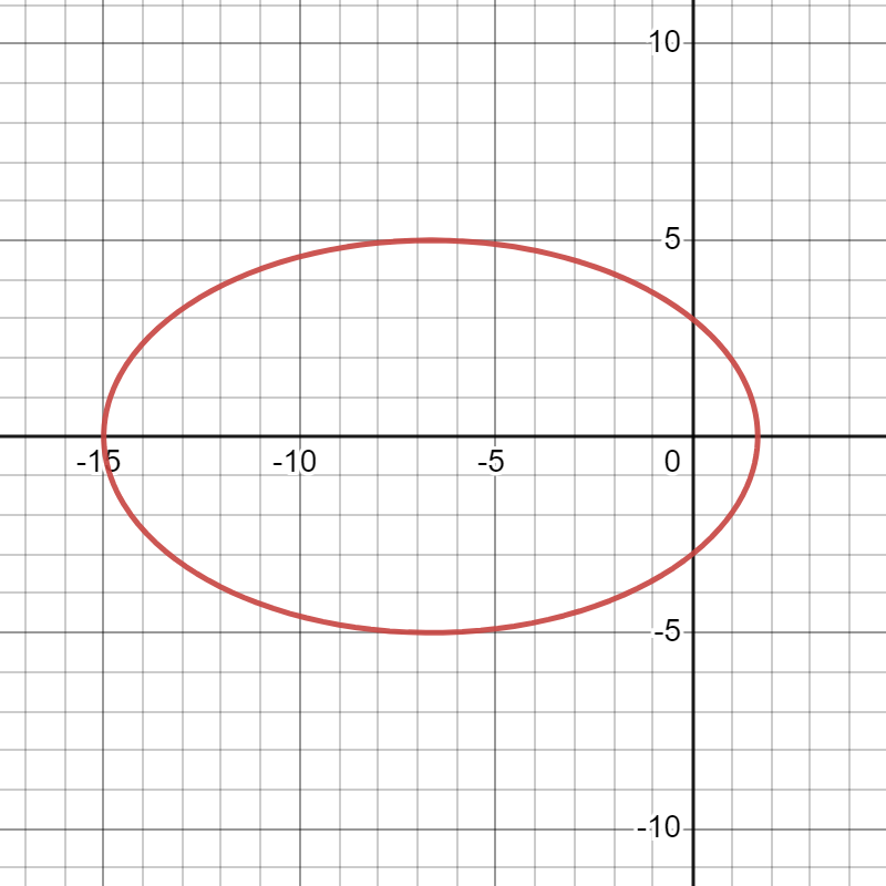
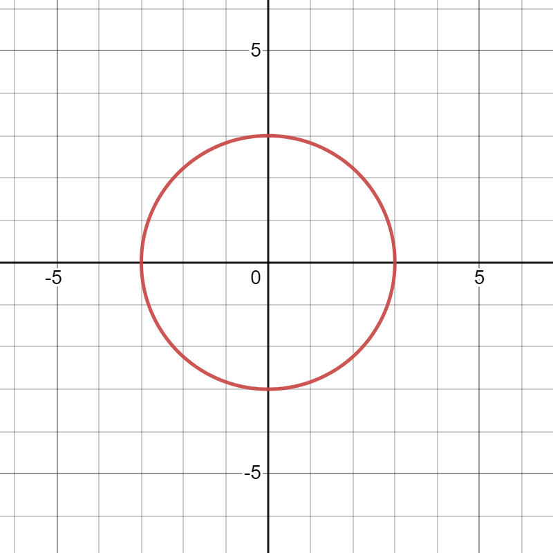
Second, I suggest setting $a=3$ and $k=0$ but altering the value of $e$ . Starting at $e=0$ , the graph is a circle. This makes complete sense: if $e=0$ , then the equation simply becomes $r=a$ , so the distance from the origin is the same for all angles. However, as $e$ increases, the original circle becomes more and more stretched out. We will prove this analytically in a later post, but it turns out that, for $0 < e < 1$ , the graph is an ellipse, and the origin is one of the foci of the ellipse. The number $e$ is called the eccentricity of the ellipse (hence the letter $e$ ).

Again, if the value of $e$ is fixed but $a$ varies, the graph becomes either larger or smaller as $a$ becomes larger or smaller.

We notice that if $0 < e < 1$ and $k=0$ , then the denominator of

$r = \displaystyle \frac{r}{1 + e \cos \theta}$

varies between $1-e$ and $1+e$ . In particular, the denominator is always positive. Therefore, the value of $r$ is least positive — the graph is closest to the origin — when the denominator is greatest. This happens when $\theta$ is a multiple of $2\pi$ . So, for example, when $\theta = 0$ , then $r = a/(1+e)$ is as close as the graph gets to the origin. Let’s call this closest distance $P$ ; in the context of a planet’s orbit around the sun, this represent perihelion. Then we have $P = \displaystyle \frac{a}{1+e}$ .

When $e=1$ , the graph switches from an ellipse to a parabola, where the origin is the focus of the parabola. For $e>1$ , the graph becomes a hyperbola. However, since we’re mostly going to be concerned with stable planetary orbits in this series, we won’t dwell too much on the case $e \ge 1$ .

Third, I suggest setting $a=3$ , $e=0.8$ , and then alter the value of $k$ . For $k=0$ , the graph is simply a single ellipse. However, by changing the value of $k$ , the graph changes into a spiral.

In the above figure, the spiral stopped “spiraling” because I had asked Desmos only to show the graph between $0 \le \theta \le 20 \pi$ . If I had changed the upper bound to something larger than $20\pi$ , the spiral would continue.

The precession in the spiral is defined to be the angular offset between each loop of the spiral. Clearly, this is a function of $k$ . To find this function, we again examine the function

$r = \displaystyle \frac{a}{1 + e \cos (1-k)\theta}$

Once again, if $0 < e < 1$ , then the denominator varies between $1-e$ and $1+e$ . In particular, the denominator is always positive. Therefore, the value of $r$ is least positive when the denominator is greatest, and the denominator is greatest when $(1-k)\theta$ is a multiple of $2\pi$ . So, for example, when $\theta = 0$ , then $r = a/(1+e)$ is as close as the graph gets to the origin.

When does the graph return to its closest point to the origin next? This would occur when $(1-k)\theta = 2\pi$ , or $\theta = \displaystyle \frac{2\pi}{1-k}$ . If $k =0$ , then the angle of closest approach to the origin would $\theta =2\pi$ , and the graph simply cycles over itself. However, if $k > 0$ , then this angle $\theta$ will be larger than $2\pi$ , thus producing a spiral. Indeed, the amount of precession would be equal to

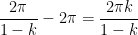
$\displaystyle \frac{2\pi}{1-k} - 2\pi = \frac{2\pi k}{1-k}$ .

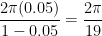
In the picture above, $k = 0.05$ . Therefore, the amount of precession would be $\displaystyle \frac{2\pi (0.05)}{1-0.05} = \frac{2\pi}{19}$ radians $\approx 18.95^\circ$ . Therefore, after 19 “leafs” of the spiral, the graph would begin to cycle on top of itself.