Solving Problems Submitted to MAA Journals (Part 6c)

The following problem appeared in Volume 97, Issue 3 (2024) of Mathematics Magazine.

Two points and are chosen at random (uniformly) from the interior of a unit circle. What is the probability that the circle whose diameter is segment lies entirely in the interior of the unit circle?

As discussed in the previous post, I guessed from simulation that the answer is . Naturally, simulation is not a proof, and so I started thinking about how to prove this.

My first thought was to make the problem simpler by letting only one point be chosen at random instead of two. Suppose that the point is fixed at a distance from the origin. What is the probability that the point , chosen at random, uniformly, from the interior of the unit circle, has the desired property?

My second thought is that, by radial symmetry, I could rotate the figure so that the point is located at . In this way, the probability in question is ultimately going to be a function of .

There is a very nice way to compute such probabilities since is chosen at uniformly from the unit circle. Let be the probability that the point has the desired property. Since the area of the unit circle is , the probability of desired property happening is

.

So, if I could figure out the shape of , I could compute this conditional probability given the location of the point .

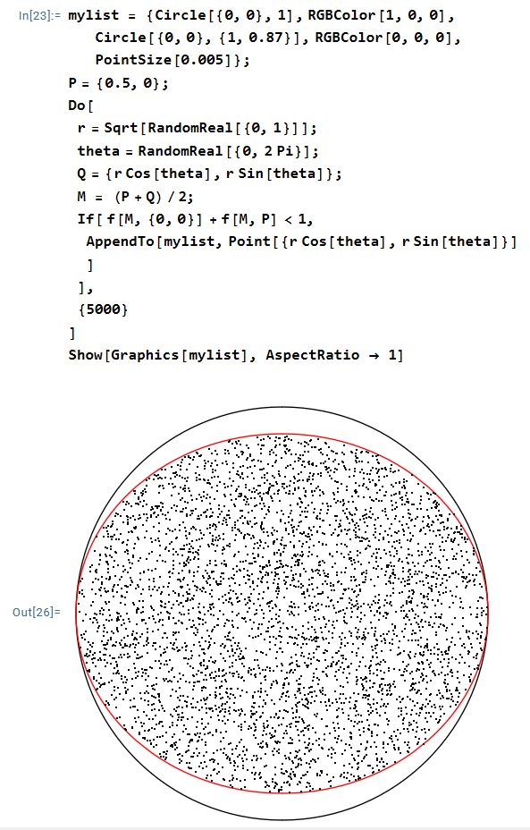
But, once again, I initially had no idea of what this shape would look like. So, once again, I turned to simulation with Mathematica. As noted earlier in this series, the circle with diameter will lie within the unit circle exactly when , where is the midpoint of . For my initial simulation, I chose to have coordinates .

To my surprise, I immediately recognized that the points had the shape of an ellipse centered at the origin. Indeed, with a little playing around, it looked like this ellipse had a semimajor axis of and a semiminor axis of about .

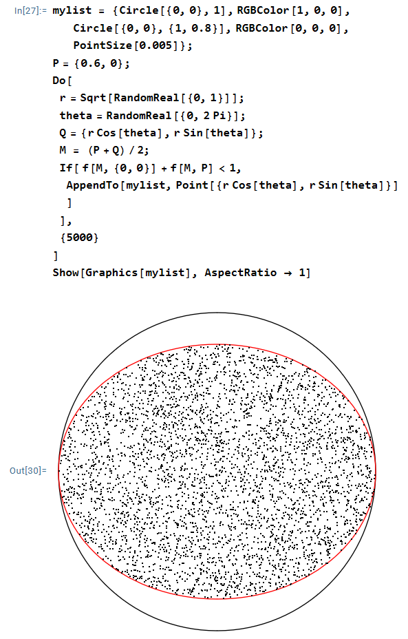
My next thought was to attempt to find the relationship between the length of the semiminor axis at the distance of from the origin. I thought I’d draw of few of these simulations for different values of and then try to see if there was some natural function connecting to my guesses. My next attempt was ; as it turned out, it looked like the semiminor axis now had a length of .

At this point, something clicked: is a Pythagorean triple, meaning that

Also, is very close to , a very familiar number from trigonometry:

So I had a guess: the semiminor axis has length . A few more simulations with different values of confirmed this guess. For instance, here’s the picture with .

Now that I was psychologically certain of the answer for , all that remain was proving that this guess actually worked. That’ll be the subject of the next post.