In this series, I’m discussing how ideas from calculus and precalculus (with a touch of differential equations) can predict the precession in Mercury’s orbit and thus confirm Einstein’s theory of general relativity. The origins of this series came from a class project that I assigned to my Differential Equations students maybe 20 years ago.
We have shown that the motion of a planet around the Sun, expressed in polar coordinates 


where 


In the previous post, I used a standard technique from differential equations to find the general solution of
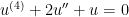
to be

However, as much as possible in this series, I want to take the perspective of a talented calculus student who has not yet taken differential equations — so that the conclusion above is far from obvious. How could this be reasonable coaxed out of such a student?
To begin, we observe that the characteristic equation is
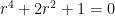
or

Clearly this has the same roots as the simpler equation 


and

The far trickier part is finding the two additional solutions. To find these, we use a standard trick/technique called reduction of order. In this technique, we guess that any additional solutions much have the form of either

where 

Doing this will require multiple applications of the Product Rule for differentiation. We already know that

We now differentiate again, using the Product Rule, to find 
![(fg)'' = ( [fg]')' = (f'g)' + (fg')'](https://s0.wp.com/latex.php?latex=%28fg%29%27%27+%3D+%28+%5Bfg%5D%27%29%27+%3D+%28f%27g%29%27+%2B+%28fg%27%29%27&bg=ffffff&fg=000000&s=0&c=20201002)


We now differential twice more to find 
![(fg)''' = ( [fg]'')' = (f''g)' + 2(f'g')' + (fg'')'](https://s0.wp.com/latex.php?latex=%28fg%29%27%27%27+%3D+%28+%5Bfg%5D%27%27%29%27+%3D+%28f%27%27g%29%27+%2B+2%28f%27g%27%29%27+%2B++%28fg%27%27%29%27&bg=ffffff&fg=000000&s=0&c=20201002)


A good student may be able to guess the pattern for the next derivative:
![(fg)^{(4)} = ( [fg]''')' = (f'''g)' + 3(f''g')' +3(f'g'')' + (fg''')'](https://s0.wp.com/latex.php?latex=%28fg%29%5E%7B%284%29%7D+%3D+%28+%5Bfg%5D%27%27%27%29%27+%3D+%28f%27%27%27g%29%27+%2B+3%28f%27%27g%27%29%27+%2B3%28f%27g%27%27%29%27+%2B+%28fg%27%27%27%29%27&bg=ffffff&fg=000000&s=0&c=20201002)


In this way, Pascal’s triangle makes a somewhat surprising appearance; indeed, this pattern can be proven with mathematical induction.
In the next post, we’ll apply this to the solution of the fourth-order differential equation.

One thought on “Confirming Einstein’s Theory of General Relativity With Calculus, Part 6f: Rationale for Method of Undetermined Coefficients III”