Confirming Einstein’s Theory of General Relativity With Calculus, Part 5a: Confirming Orbits under Newtonian Mechanics with Calculus

In this series, I’m discussing how ideas from calculus and precalculus (with a touch of differential equations) can predict the precession in Mercury’s orbit and thus confirm Einstein’s theory of general relativity. The origins of this series came from a class project that I assigned to my Differential Equations students maybe 20 years ago.

We previously showed that if the motion of a planet around the Sun is expressed in polar coordinates $(r,\theta)$ , with the Sun at the origin, then under Newtonian mechanics (i.e., without general relativity) the motion of the planet follows the differential equation

$u''(\theta) + u(\theta) = \displaystyle \frac{1}{\alpha}$ ,

where $u = 1/r$ and $\alpha$ is a certain constant. We will also impose the initial condition that the planet is at perihelion (i.e., is closest to the sun), at a distance of $P$ , when $\theta = 0$ . This means that $u$ obtains its maximum value of $1/P$ when $\theta = 0$ . This leads to the two initial conditions

$u(0) = \displaystyle \frac{1}{P} \qquad \hbox{and} \qquad u'(0) = 0$ ;

the second equation arises since $u$ has a local extremum at $\theta = 0$ .

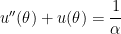
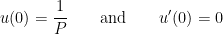
In the next few posts, we’ll discuss the solution of this initial-value problem. Today’s post would be appropriate for calculus students, which is confirming that

$u(\theta) = \displaystyle \frac{1 + \epsilon \cos \theta}{\alpha}$

solves this initial-value problem, where $\epsilon = \displaystyle \frac{\alpha-P}{P}$ . Since $r$ is the reciprocal of $u$ , we infer that

$r = \displaystyle \frac{\alpha}{1 + \epsilon \cos \theta}$ .

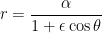
As we’ve already seen in this series, this means that the orbit of the planet is a conic section — either a circle, ellipse, parabola, or hyperbola. Since the orbit of a planet is stable and $\epsilon = 0$ is extremely unlikely, this means that the planet orbits the Sun in an ellipse, with the Sun at one focus of the ellipse.

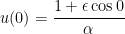
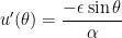
So, for a calculus student to verify that planets move in ellipses, one must check that

$u(\theta) = \displaystyle \frac{1 + \epsilon \cos \theta}{\alpha}$

is a solution of the initial-value problem

$u''(\theta) + u(\theta) = \displaystyle \frac{1}{\alpha}$ ,

$u(0) = \displaystyle \frac{1}{P}$ ,

$u'(0) = 0$ .

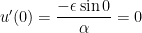
The second line is easy to check:

$u(0) = \displaystyle \frac{1 + \epsilon \cos 0}{\alpha}$

$= \displaystyle \frac{1 + \epsilon}{\alpha}$

$= \displaystyle \frac{1 + \displaystyle \frac{\alpha-P}{P}}{\alpha}$

$= \displaystyle \frac{1}{\alpha} \frac{P + \alpha - P}{P}$

$= \displaystyle \frac{1}{\alpha} \frac{\alpha}{P}$

$= \displaystyle \frac{1}{P}$ .

The third line is also easy to check:

$u'(\theta) = \displaystyle \frac{-\epsilon \sin \theta}{\alpha}$

$u'(0) = \displaystyle \frac{-\epsilon \sin 0}{\alpha} = 0$ .

To check the first line, we first find $u''(\theta)$ :

$u''(\theta) = \displaystyle \frac{-\epsilon \cos \theta}{\alpha}$ ,

so that

$u''(\theta) + u(\theta) = \displaystyle \frac{-\epsilon \cos \theta}{\alpha} + \frac{1 + \epsilon \cos \theta}{\alpha} = \frac{1}{\alpha}$ ,

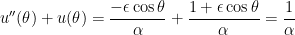
thus confirming that $u(\theta) = \displaystyle \frac{1 + \epsilon \cos \theta}{\alpha}$ solves the initial-value problem.

While the above calculations are well within the grasp of a good Calculus I student, I’ll be the first to admit that this solution is less than satisfying. We just mysteriously proposed a solution, seemingly out of thin air, and confirmed that it worked. In the next post, I’ll proposed a way that calculus students can be led to guess this solution. Then, we talk about finding the solution of this nonhomogeneous initial-value problem using standard techniques from differential equations.

One thought on “Confirming Einstein’s Theory of General Relativity With Calculus, Part 5a: Confirming Orbits under Newtonian Mechanics with Calculus”

Confirming Einstein’s Theory of General Relativity With Calculus, Part 5a: Confirming Orbits under Newtonian Mechanics with Calculus

Published by John Quintanilla

One thought on “Confirming Einstein’s Theory of General Relativity With Calculus, Part 5a: Confirming Orbits under Newtonian Mechanics with Calculus”

Leave a comment Cancel reply

Share this:

Related

Published by John Quintanilla

One thought on “Confirming Einstein’s Theory of General Relativity With Calculus, Part 5a: Confirming Orbits under Newtonian Mechanics with Calculus”

Leave a comment Cancel reply